1. Introduction

The mathematical formulation of the conservation laws of mass, momentum and energy is the first step in the modelling of fluid flow problems by the finite element method. Thus, we obtain the Navier-Stokes equations, convection-diffusion transport equations, and the Euler equations, convection transport equations. In this first step of resolution, it is advisable to make a judicious choice of the form and the independent variables. Indeed, there are several possible choices [1], mainly: the non-conservative form, the conservative form in entropic variables and the conservative form. Physically, the conservative formulation is best suited to the fact that equations fluid dynamics are solved by perfectly respecting the laws of physics; in addition the boundary conditions are directly imposed on the physical variables.

The finite element method is one of the most powerful numerical methods conceived to date. The characteristics that have led to its popularity include: ease of modelling complex shape geometries, natural processing of differential-type boundary conditions, and the possibility of being programmed in the form of software adaptable to the processing of a wide range of problems. The classical formulation of the finite element method is based on the Galerkin weighted residual method. Galerkin’s formulation has proved to be extremely effective in applying structural mechanics problems and in other situations such as problems governed by diffusion equations. The reason for this success is that in application to problems governed by elliptic or parabolic partial differential equations, Galerkin’s finite element method leads to symmetric stiffness matrices. The advantages of the Galerkin’s finite element method in solving the problems of structural mechanics and diffusion transport are not directly exploitable for the modelling of fluid flow problems, particularly in the simulation of transport phenomena dominated by convection. A major difficulty arose because of the presence of convective terms in the mathematical formulation when using a kinematic description other than the Lagrangian description as this is practically always the case in fluid mechanics. In practice, Galerkin’s numerical solutions for dominant convective problems are frequently polluted by non-physical oscillations which can only be eliminated by considerably refining the mesh, or in the case of transient greatly reducing the time step. This, of course, compromises the very usefulness of the Galerkin method and has motivated the development of alternative methods that exclude the presence of non-physical oscillations independently of any mesh refinement or time step [2-6].

This article proposes elements of answer to these points. The objective analysis of the choice of form and variables independent of convection-diffusion transport equations; justifies our choice of the conservative form using conservative variables to solve the Navier-Stokes and Euler equations. The variational form used is based on Galerkin’s weighted residual method. For the flow problems of dominant convection or pure convection fluids, the variational form used is based on a Petrov-Galerkin type formulation. Emphasis is placed on the development and implementation of these two types of variational formulations.

2.       Mathematical formulation

We recall in this section the equations of the dynamics of compressible and viscous fluids. These equations express conservation laws of mass, momentum and energy. By identifying conservative variables, namely the density , the momentum per unit volume , and the total energy per unit volume , as the independent variables, the Navier-Stokes equations, in conservative form and dimensionless, are written:

where , , , ,  and  represent respectively: velocity, pressure, heat flux, energy source, external force and tensor of viscous stresses. The heat flux and the pressure are expressed, in non-dimensional form, as a function of the temperature and of the density by the Fourier law and the equation of a perfect gas, respectively:

and

where , ,  and  represent respectively: Reynolds number, Prandlt number, specific heat ratio and temperature. On the other hand, the tensor of viscous stresses  is given by the relation:

where  is the identity matrix. Temperature and velocity are related to conservative variables by the following relationships:

The substitution of equation (6) in equation (4) decomposes the viscous stress tensor in the following form:

where

On the other hand, the substitution of equations (5) and (6) in equations (2) and (3) makes it possible to express the heat flux and the pressure, as a function of conservative variables ( ,  and ), respectively by the following relationships:

and

Equations (1) are strongly nonlinear, their mathematical study is a great challenge and their numerical resolution is not easy. The variational formulation as well as the finite element approximation must respect, inter alia, the implicit condition that temperature, pressure and density must be positive.

Let  be the vector of conservative variables:

the system of equations (1) can be written in the vector form:

where  and  are respectively the convection and diffusion fluxes in the  direction, and  is the source vector. It is also interesting to write the system (1) in the quasi-linear form:

with  the Jacobian matrices of the convection fluxes such that  and  the diffusion matrices such as

.

The flow problems of non-viscous fluids, governed by the Euler equations, are a special case of the flow of viscous fluids. To find the Euler equations, we suppress the viscous terms in the Navier-Stokes equations.

The Euler equations can be written respectively in the vector form and the quasi-linear form, as follows:

2.1.  Boundary and Initial Conditions

We consider external and internal flows, the domain of calculation is denoted  of boundary .

Inlet boundary condition

The flow is considered uniform:

where  is the angle of attack and  is the Mach number at infinity.

Wall boundary condition

The condition of adhesion ( ) is imposed in the case of viscous fluid flow problems and a sliding condition ( ) in the case of flow problems of non-viscous fluids. In addition, one imposes either a natural condition of Neumann type on the temperature (adiabatic wall): , or a uniform distribution of the temperature  in order to represent a thermal equilibrium condition to the wall; which amounts to imposing the Dirichlet condition: . In the case of a uniform temperature distribution, for Mach numbers less than 3, we take  equal to the stagnation temperature:

Since  is unknown, the boundary condition  is non-linear. During the resolution, the value of the energy at the wall must therefore be continuously updated as a function of the density.

Outlet boundary condition

Two cases must be distinguished. If the local Mach number is less than unity, subsonic regime, then at least one condition at the Dirichlet boundary (on density or on pressure or on total energy) is required. If the local Mach number is greater than unity, supersonic regime, then no boundary condition is necessary.

The initial conditions are:

3.       Galerkin formulation

Let  be a bounded one of the Euclidean space , of boundary . In order to determine a solution numerically, we cancel the projection of the system of equations (1) onto a set of weighting functions according to the Galerkin method. The weighting functions of the conservative variables ( , , ) are denoted by  ,  and , respectively. By multiplying the equations (1) in turn by weighting functions, we have:

where  denotes the scalar product in , and:

The integration by parts of the terms of diffusion makes it possible to reduce the derivation order from two to one. The appearance of contour integrals can be used to impose natural boundary conditions such as adiabatic wall conditions and sliding conditions. Using vector notation (10), the variational formulation (12) is written as follows:

with  the vector of the weighting functions. Also, using the quasi-linear form (11), we establish the following variational formulation:

4.       Petrov-Galerkin formulation

4.1.  Artificial Viscosity

The method of artificial viscosity used consists in replacing the dynamic viscosity  by:

where  is defined in a similar way as artificial diffusion widely used in finite difference schemes:

where  is the size of the element,  is the weighting coefficient of the viscosity and  is the local Reynolds number:

The function  is particularly sensitive to zones with dominant convection; it is defined as follows:

Thus, the modified system of equations includes an artificial viscosity term whose importance depends on the function  and the weighting coefficient . By experience, it is necessary to increase the viscosity in the zones with dominant convection (ie local Reynolds number is large). The effect of this artificial viscosity is to create additional energy dissipation, thus guaranteeing the positivity of temperature, density and pressure. This method has the advantage of being easy to implement and does not require any additional calculations, however it has the disadvantage of containing an arbitrary coefficient  whose value influences the quality of the solution. We essentially use this method to quickly obtain a solution, although diffusive, converges towards the final solution. This solution subsequently serves to initialize the stabilized formulation by Petrov-Galerkin finite element method which we describe in the following section.

4.2.  SUPG Method

The Petrov-Galerkin formulation that we use is a variant of the Streamline Upwind Petrov-Galerkin (SUPG) method [2-6]. The SUPG method is based on a Petrov-Galerkin formulation, this method is widely used for the resolution of convection-diffusion transport equations. As already mentioned in the introduction, when convection dominates, the use of the Galerkin method generates non-physical oscillations which can only be eliminated by considerably refining the mesh, or by greatly reducing the time step in the transient case. The SUPG method consists in adding an additional perturbation term to the Galerkin standard formulation. On the other hand, the use of the Petrov-Galerkin formulation amounts to modifying the weighting functions of the Galerkin type by weighting functions having more weight upstream; thus introducing artificial diffusion in the direction of the flow. The variational formulation (13) is modified as follows:

where  is an element of the triangulation of the computational domain . The matrix , for the conservative form using the conservative variables, is written in the following form:

In equation (14), the coefficients  represent the elements of the Jacobian matrix of the geometric transformation of the real element to the reference element. The operator  applied to a matrix  defines its absolute value  by: , where  and  are respectively the matrices of the eigenvectors and the eigenvalues of . In order to compute  from equation (14) we must obtain the absolute values of matices . The definition of the matrix  therefore requires the solving of a problem with eigenvalues. It should also be recalled that the Jacobian matrices  and  of the convection flux in direction i with respect to the conservative and non-conservative variables respectively are connected by the following relation:

with

In two dimensions, the vectors of conservative and non-conservative variables are written respectively:

Analytically, the matrices  and  can be obtained in the two-dimensional case

and

with . The expressions of  and  are given in the two-dimensional case by:

and

with  the velocity of sound.

5.       Resolution algorithm

The spatial-temporal discretization of the variational problem leads to the solution of a system of algebraic equations of the form:

This system of equations has several types of non-linearities. Some are due to convective terms, others are related to the compressibility of the fluid. In addition, the use of the Petrov-Galerkin method introduces strong non-linearities. Given the set of nonlinear equations, stability of the solution and convergence, the use of a robust algorithm is therefore crucial. Given its convergence properties, the Newton-Raphson algorithm coupled to the chosen implicit time scheme can be effective in solving this problem. However, in the present situation, the implementation of the Newton-Raphson method requires the calculation of the first variations of all the functional ones present in the formulation. These exact analytical expressions are difficult to obtain, especially in the presence of a stabilization method. To solve the problem, we use a variant of the GMRES algorithm [7]. To accelerate the convergence of the GMRES algorithm, pre-conditioning techniques are used.

6.       Numerical results

A first series of numerical tests concerning external flows of viscous and non-viscous fluids around a NACA0012 profile was carried out to validate the methods described above. The mesh used comprises 8150 elements. This mesh is illustrated in figure 1, with an enlargement around the profile NACA0012 in figure 2.

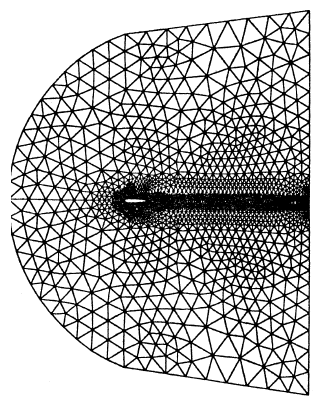Figure 1: Mesh over the entire domain

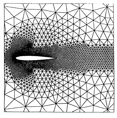Figure 2: Mesh around profile NAC0012

Viscous flow

The first problem presented is a viscous flow at  and  with a zero angle of attack. The initial solution used is a uniform field except at the wall. The resolution strategy consists in fixing the Reynolds and Mach numbers to their maximum values and to solve the problem over 200 time steps ( ) with an artificial viscosity ( ). The resulting solution serves as the initial field for the computation sequence in which the artificial viscosity is canceled by imposing ( ), and the SUPG method is applied until converges of the temporal scheme. The iso-Mach and iso-density curves are shown in figures. 3a and 3b. The pressure coefficients  on the profile are compared in figure 3c with those obtained by a finite element method using non-conservative variables [8].

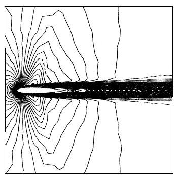Figure 3a: Iso-Mach lines

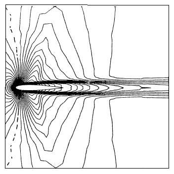Figure 3b: Iso-density lines

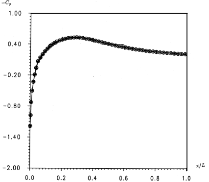Figure 3c: Pressure coefficient

Non-viscous flow

The Euler equations are now solved for  and for an angle of attack of  degrees; these conditions are similar to those defined in the [6, 9]. The initial solution used is a uniform field except at the wall where we impose the normal component of the velocity at zero. The resolution strategy consists in using the SUPG method from the beginning of the resolution to the convergence in time. The mesh is identical to that shown above. The iso-Mach and iso-pressure curves are shown in FIGS. 4a and 4b. The presence of two zones of low pressure followed by normal shocks is noted, as can be expected conventionally in transonic flow. FIG. 4c shows the evolution of the pressure coefficient along the profile, these results are compared with those obtained by [6, 10] with Roe schemes in finite volumes. We note that for our results the shocks are well defined on the intrados as on the extrados. Obviously, the resolution of shocks can be further improved by using mesh adaptation methods.

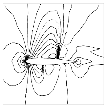Figure 4a: Iso-Mach lines

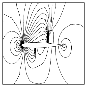Figure 4b: Iso-pressure lines

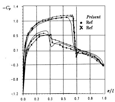Figure 4c: pressure coefficient

The same problem is then dealt with for an angle of attack of  degrees. The iso-Mach, iso-pressure curves and the distribution of the pressure coefficient for this test case are presented in figures 4d, 4e and 4f. The presence of a strong shock on the extrados is noted.

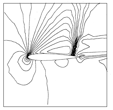Figure 4d: iso-Mach lines

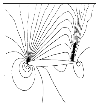Figure 4e: iso-pressure lines

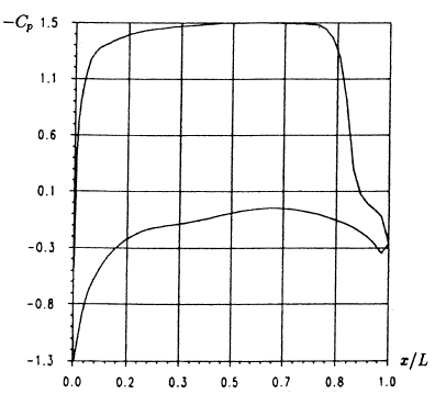Figure 4f: pressure coefficient

Flow around a half cylinder

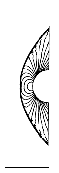
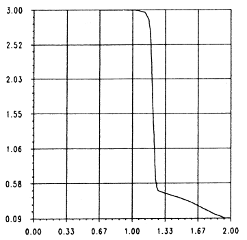
The simulation of this flow is aimed at validating the methods described above in the case of supersonic flows. The test consists of simulating the flow around a half cylinder at a Mach number of  without angle of incidence. The calculation domain and the boundary conditions used are illustrated in figure 5a. The resolution strategy is identical to that used in the previous example. In addition, the mesh has been refined during the resolution. The final mesh consists of 15 148 elements. The iso-pressure is shown in figure 5b, this figure is very similar to that presented by [11]. A section of the iso-Machs at the line of symmetry is shown in figure 5c.

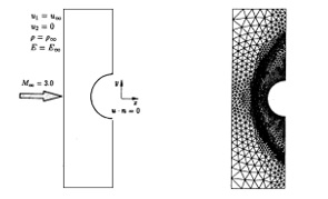Figure 5a: Meshing around a half cylinder Figure 5b: Iso-pressure lines Figure 5c: iso-Mach section at the line of symmetry

7.       Conclusion

We have presented a finite element method for solving the Navier-Stokes and Euler equations using conservative variables and a Petrov-Galerkin variational formulation. Particular emphasis was placed on the effective definition and implementation of the Stabilization Matrix. The use of the pre-conditioned GMRES algorithm with an adequate resolution strategy allows a relatively fast convergence. The numerical results obtained show that the present finite element method gives results at least as good as those obtained with other methods. However, it seems imperative for shock problems to use a conservative method; the use of conservative variables is indeed an essential ingredient. The condition of the conservation of the mass at the level of each element is also respected.

1. J.R. Hughes, G. Scovazzi and T.E. Tezduyar. ”Stabilized methods for compressible flows.” Journal of Scientific Computing, 43, 343-368, 2010.
2. de Frutos J., B. Garcia-Archilla, V. John and J. Novo, ”An adaptive SUPG method for evolutionary convection–diffusion equations.” Computer Methods in Applied Mechanics and Engineering, 273, 219-237, 2014.
3. Ganesan S. ”An operator-splitting Galerkin/SUPG finite element method for population balance equations: Stability and convergence.” ESAIM: Mathematical Modeling and Numerical Analysis (M2AN), 46, 1447-1465, 2012.
4. John V. and Novo J., “”Error analysis of the SUPG finite element discretization of evolutionary convection-diffusion-reaction equations.” SIAM Journal on Numerical Analysis, 49, (3), 1149-1176, 2011.
5. Wang, W. K. Anderson, J. T. Erwin, and S. Kapadia, ”Discontinuous Galerkin and Petrov Galerkin methods for compressible viscous flows.” Computers & Fluids, (100), 13-29, 2014.
6. K. Anderson, B. R. Ahrabi, and J. C. Newman. ”Finite Element Solutions for Turbulent Flow over the NACA 0012 Airfoil.” AIAA Journal, 54, (9), 2688-2704, 2016.
7. Saad and M. H. Schultz, ”GMRES: a generalized minimal residual algorithm for solving nonsymmetric linear systems.” SIAM J. Sci. Stat. Comp., 7, 856-869, 1986.
8. Fortin, H. Manouzi and A. Soulaimani. ”On finite element approximations and stabilization methods for compressible viscous flows.” International Journal of Numerical Methods in fluids, 17, (6), 477-499, 1993.
9. Rizzi and H. Viviand editors, ”Numerical methods for the computation of inviscid transonic flows with shock waves, a GAMM-Workshop.” Volume 3 of notes on numerical fluid mechanics, Vieweg Verlag, 1981.
10. J. Barth. ”Computational fluid dynamics, on unstructured grids and solvers.” von Karman Institute for fluid dynamics, NASA Ames Research Center, USA, Lecture Series 1990-03, March 5-9, 1990.
11. Johan, T.J.R. Hughes and F. Shakib, ”A globally convergent matrix-free algorithm for implicit time-marching schemes arising in finite element analysis in fluids.” Computer Methods in Applied Mechanics and Engineering, 87, 281-304, 1991.

(Click to view)

(Click to view)