1. Introduction

Frequent pattern mining plays an important role in mining associa- tions [1, 2, 3, 4], which are quite useful for decision making. For instance, for the supermarket management, the association rules are used to decide, how to place merchandise on shelves, what to put on sale, as well as how to design coupons to increase the profit, etc. In general, by the frequent pattern mining [5, 6, 7, 8], we are required to find a frequent pattern, which is in fact a subset of items supported (or say, contained) by most of transactions. Here, by a transaction, we mean a set of attributes or items.

In this paper, we study a more challenging problem, the so- called single package design problem (SPD for short [2, 3, 9, 10]), defined below:

• A set of attributes (items, or activities):

A = {a₁, …, a_m},

• A query log:

Q = {q₁, . . . q_n},

where each q_i = c_i1c_i2 . . . c_im with each c_{i j} ∈ {0, 1, *} (i = 1,

. . . , n, j = 1, . . . , m).

• In q_i, whether a_j is chosen, depends on the value of c_{i j}. That is, if c_{i j} = 1, a_j is selected; if c_{i j} = 0, a_j is not selected; otherwise, c_{i j} = ‘*’ means ‘don’t care’.

Our purpose is to find a bit string τ = τ₁ … τ_m that satisfies as many queries q^′s in Q as possible. We say, τ satisfies a q_i = c_i1c_i2 . . . c_im if for each j (1 ≤ j ≤ m) the following conditions are satisfied:

c_{i j} = 1 → τ _j = 1,

c_{i j} = 0 → τ _j = 0,

c_{i j} = ‘*’ → τ _j = 1 or 0.

A τ is referred to as a package. If it is able to satisfy a maximum subset of queries, we call it a most popular package. For instance, for the above vacation package, a query in a log can be created by specifying yes, no, or ‘don’t care’ for each activity by a client. Then, the design of a most popular package is essentially to decide a subset of such activities to satisfy as many queries’ requirements (normally according to a questionnaire) as possible. It is a kind of extension to mining association rules in data mining [5], but more general and therefore more useful in practice.

This problem has been investigated by several researchers [9, 10]. The method discussed in [10] is an approximation algorithm, based on the reduction of SPD to MINSAT [11], by which we seek to find a truth assignment of variables in a logic formula (in con- junctive normal form) to minimize the number of satisfied clauses. This is an optimization version of the satisfiability problem [12]. In [9], a kind of binary trees, called signature trees [13, 14, 15] for signature files [16, 17, 18, 19, 20], is contructed to represent query logs. Its worst-case time complexity is bounded by O(n2^m).

In this paper, we address this issue and discuss two different algorithms to solve the problem. By the first method, we will construct a binary tree over a query log in a way similar to [9], but establishing a kind of heuristics to cut off futile branches. Its aver- age time complexity is bounded by O(nm² + m2^m/2). The second algorithm is based on a compact representation of the query log, by which all the query bit strings are organized into a trie-like graph G. Searching G bottom-up recursively, we can find a most popular package in O(n²m³(log₂ nm)^log2 nm) time.

The remainder of the paper is organized as follows. First, we show a simple example of the SPD problem in Section 2. Then, Section 3 is devoted to the discussion of our first algorithm for solving the SPD problem, as well as its time complexity analysis. Next, in Section 4, we discuss our second algorithm in great detail. Finally, we conclude with a summery and a brief discussion on the future work in Section 5.

2. An example of SPD

In this section, we consider a simple SPD shown in Table 1, which contains a query log with n = 6 queries, and m = 6 attributes (ac- tivities), created based on a questionnaire on customers’ favourites. For example, the query q₆ = a₁₁a₁₂ . . . a₁₆ = (*, 1, *, 0, *, 1) in Table 1 shows that ride and boating are q₆’s favourites, but hike is not. In addition, q₆ does not care about whether hot spring, glacier or airline is available or not.

Table 1: A query log Q

query	hot spring	ride	glacier	hike	airline	boat- ing
q1	1	*	0	*	1	*
q2	1	0	1	*	*	*
q3	*	0	0	1	1	*
q4	0	*	1	*	1	*
q5	*	0	0	*	*	0
q6	*	1	*	0	*	1

For this small query log, a most popular package can be found, which contains three items: hot spring, hiking, airline, and is able to satisfy a maximum subset of queries: q₁, q₃, q₅.

3. The First Algorithm

In this section, we discuss our first algorithm. First, in Section 3.1, we give a basic algorithm to provide a discussion background. Then, we describe this algorithm in great detail in Section 3.2. The analysis of the average running time is conducted in Section 3.3.

3.1. Basic algorithm

We first describe a basic algorithm to facilitate the subsequent dis- cussion, which is in fact an extension of an algorithm discussed in [15]. The main idea behind it is the construction of a binary tree T over a query log Q. The algorithm works in two steps. In the first step, a signature-tree-like structure is built up, referred to as a search-tree. Then, in the second step, the search-tree is explored to find a most popular package.

Given a set of attributes: A = {a₁, a₂, . . . , a_m} and a query log: Q = {q₁, . . . , q_n} over A. Denote by q_i[ j] the value of the jth attribute a_j in q_i (i = 1, . . . , m). Then, the binary tree T can be constructed as follows.

1. First, for the whole Q, create root of T . j :=
2. For each leaf node v of the current T , denote by s_v the subset of queries represented by v. For query q_i (∈ s_v ), if q_i[1] = ‘0’, we put q_i into the left branch. If q_i[1] = ‘1’, it is put into the right branch. However, if q_i[1] = ‘*’, we will put it in both left and right branches, showing a quite different behavior from a traditional signature tree construction [15].
3. j := j + If j ¿ m, stop; otherwise, go to (2).

For example, for the query log given in Table 1, we will con- struct a binary search tree as shown in Fig. 1.

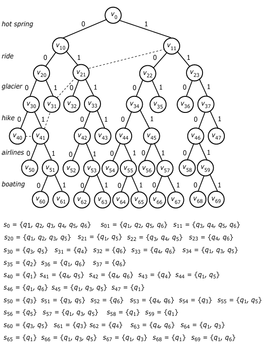
In Fig. 1, we use s_u to represent the subset of queries associated with u. In terms of the corresponding attribute a, s_u is decomposed into two subsets: s_u(a) and s_u(¬a), where for each q ∈ s_u(a) we have q[a] = 1 and for each q^′ ∈ s_u(¬a) q^′[a] = 0. In general, s_u(¬a) is represented by u’s left child while s_u(a) is represented by u’s right child.

For example, the subset of queries associated with v₁₁ is s₁₁ = {q₃, q₄, q₅, q₆}. According to attribute ‘ride’, s₁₁ is split into two subsets respectively associated with its two children (v₂₂ and v₂₃): s₂₂ = {q₃, q₄, q₅} and s₂₃ = {q₄, q₆}. In addition, we can also see that among all the leaf nodes the subset s₆₆ (= {q₁, q₃, q₅}) associated with v₆₆ is of the largest size. Then, the labels along the path from the root to it spell out a string 100110, representing a most popular package: {hot spring, hiking, airlines}.

The computational complexity of this process can be analyzed as follows.

First, we notice that in the worst case an search-tree can have O(2^m) nodes. Since each node is associated with a subset of queries, we need O(n) time to determine its two children. So, the time for constructing such a tree is bounded by O(n2^m). The space require- ment can be slightly improved by keeping only part of the search tree in the working process. That is, we need only to maintain the bottom frontier (i.e., the last nodes on each path at any time point during the construction of T .) For example, nodes v₄₀, v₄₁, v₃₁, and v₂₁ (see the dashed lines in Fig. 1) make up a bottom frontier at a certain time point. At this point, only these nodes are kept around. However, for each node v on a bottom frontier, we need to keep the bit string along the path from root to v to facilitate the recognition of the corresponding best package. In the worst case, the space overhead is still bounded by O(n2^m).

3.2. Algorithm based on priority-first search

The basic algorithm described in the previous section can be greatly improved by defining a partial order over the nodes in the search tree T to cut off futile paths. For this purpose, we will associate a key with each node v in T , which is made up of two values: <|s_v|, l_v>, where |s_v| is the subset of queries associated with v and l_v is the level of v. (Here, we note that the level of the root is 0, the level of the root’s children is 1, and so on.) In general, we say that a pair <|s_v|, l_v> is larger than another pair <|s_u|, l_u> if one of the following two conditions is satisfied:

• |s_v| > |s_u|, or
• |s_v| = |s_u|, but l_v ¿ l_u.

In terms of this partial order, we define a max-priority queue H for maintaining the nodes of T to control the tree search, with the following two operations supported:

• extractMax(H) removes and returns the node of H with the largest pair.
• insert(H, v) inserts the node v into the queue H, which is equivalent to the operation H := H ∪ {v}.

In addition, we utilize a kind of heuristics for efficiency, by which each time we expand a node v, the next attribute a chosen among the remaining attributes should satisfy the following conditions:

1. |s_v(a)| – |s_v(¬a)| is
2. In the case that more than one attributes satisfy condition (1), choose a from them such that the number of queries q in s_v with q[a] = ‘*’ being minimized (the tie is broken )

Using the above heuristics, we can avoid as many useless branches as possible.

By using the priority queue, the exploration of T is not a DFS (depth-first search) any more. That is, the search along a current path can be cut off, but continued along a different path, which may lead to a solution quickly (based on an estimation made according to the pairs associated with the nodes.) This is because by extractMax(H) we always choose a node with the largest possibility leading to a most popular package.

Algorithm 1: PRIORTY-SEARCH(Q, A)                                              

Input  :a query log Q.

Output :a most popular package P.

the pair for root is set to be <|Q|, 0>; i := 0; inset(H, root); (*root represents the whole Q.*) while i ≤ m do

v := extractMax(H); (*recall that the pair associated

with v is <|s_v|, l_v>.*)

if i = m then

return the package represented by the path from

root to v;

recognize a next attribute a from A according to

heuristics;

generate left child v_l of v, representing s_v(¬a); create left child v_r of v, representing s_v(a);

the pair of v_l is set to be <|s_v(¬a)|, l + 1>; the pair of v_r is set to be <|s_v(a)|, l + 1>; insert(H, v_l); insert(H, v_r);

i := l_v + 1;

The procedure is given in Algorithm 1. This is in fact a tree search controled by using a priority queue, instead of a stack. First, the root is inserted into the priority queue H and its key (a pair of values) is set to be <|Q|, 0>. Then, we will go into a while-loop, in each iteration of which we will extract a node v from the priority queue H with the largest key value (line 4), that is, with the largest number of queries represented by v and at the same time on the deepest level (among all the nodes in H). Then, the subset of queries represented by v will be split (see lines 7 and 8) according to a next attribute chosen in terms of the heuristics described above (line 7). Next, two children of v, denoted respectively as v_l and v_r, will be created (see lines 8 and 9). and their keys are calculated (lines 10 and 11). In line 12, these two children are inserted into H. Finally, we notice that i is used to record the level of the currently encountered node. Thus, when i = m, we must get a most popular package.

The following example helps for illustration.

Example 1. 1 In this example, we show the first three steps of computation when applying the algorithm PRIORITY-SEARCH( ) to the query log given in Table 1. For simplicity, we show only the nodes in both H and T for each step. In addition, the priority queue is essentially a max-heap structure [21], represented as a binary tree.

In the first step, (see Fig. 2(a)), the root (v₀) of T is inserted into H, whose pair is <6, 0>. It is because the root represents the whole query log Q which contains 6 queries and is at level 0. Then, in terms of attribute glacier (selected according to the heuristics), Q is split into two subsets (which may not be disjoint due to possible ‘*’ symbols in queries), which are stored as v₀’s two child nodes: v₁₀ and v₁₁ with s_v10 = {q₁, q₃, q₅, q₆} and s_v11 = {q₂, q₄, q₆}. Then, v₁₀ with pair <4, 1> and v₁₁ with <3, 1> will be inserted into H.

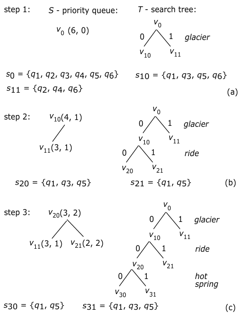
In the second step (see Fig. 2(b)), v₁₀ with pair <4, 1> will be extracted from H. This time, in terms of the heuristics, the selected attribute is ride, and s_v10 will accordingly be further divided into two subsets, represented by its two children: v₂₀ with s_v20 = {q₁, q₃, q₅} and v₂₁ with s_v21 = {q₁, q₅}. Their pairs are respectively <3, 2> and <2, 2>.

In the third step (see Fig. 2(c)), v₂₀ with pair <3, 2> will be taken out from H. According to the selected attribute hot spring, sv20 will be divided into two subsets, represented respectively by its two children: v₃₀ with s_v30 = {q₁, q₅} and v₃₁ with s_v31 = {q₁, q₃, q₅}.

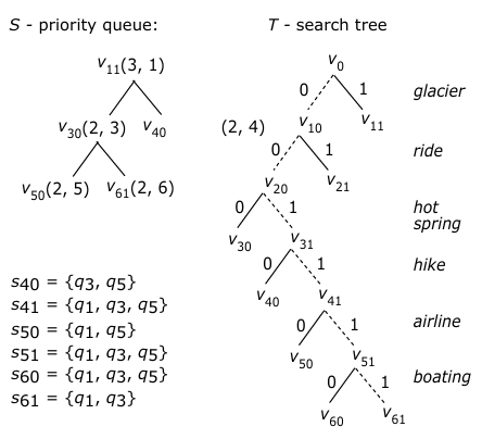
The last step of the computation is illustrated in Fig. 3, where special attention should be paid to node v₆₀, which is associated with a subset of queries: {q₁, q₃, q₅}, larger than any subset in the current priority queue H. Then, it must be one of the largest subset of queries which can be found since along each path the sizes of subsets of queries must be non-increasingly ordered. Now, by checking the labels along the path from the root to v₆₀, we can easily recognize all the attributes satisfying the queries in this subset. They are {hot spring, hiking, airline}. Since {q₁, q₃, q₅} is a maximum subset of satisfiable queries, this subset of attributes must ba a most popular package.

By this example, a very important property of T can be observed. That is, along each path, the sizes of subsets of queries (represented by the nodes) never increase since the subset of queries represented by a node must be part of the subset represented by its parent. Based on this property, we can easily prove the following proposition.

Proposition 1. Let Q be a query log. Then, the subset of attributes found in Q by applying the algorithm PRIORITY-SEARCH( ) to Q must be a most popular package.

Proof. Let v be the last node created (along a certain path). Then, the pair associated with v will have the following properties:

• l_v = m, and
• |s_v| is the largest among all the nodes in the current H.

Since the sizes of subsets of queries never increase along each path in T , s_v must be a maximum subset of queries which can be satisfied by a certain group of attributes. One such a group can be simply determined by the labels on the path from root to v. This completes the proof.

The computation shown in Example 1 is super efficient. Instead of searching a binary tree of size O(2^m) (as illustrated in Fig. 1), the algorithm PRIORITY-SEARCH( ) only explores a single root-to-leaf path, i.e., the path represented by dashed edges in Fig. 3). However, in general, we may still need to create all the nodes in a complete binary tree in the worst case.

Then, we may ask an interesting question: how many nodes need to be generated on average?

In the next subsection, we answer this question by giving a probabilistic analysis of the algorithm.

3.3. Average time complexity

From Fig. 2 and 3, we can see that for each internal node encoun- tered, both of its child nodes will be created. However, only for some of them, both of their children will be explored. For all the others, only one of their children is further explored. For ease of explanation, we call the former 2-nodes while the latter 1-nodes. We also assume that in T each level corresponds to an attribute.

Let a = a₁a₂ . . . a_m be an attribute sequence, along which the tree T is expanded level-by-level. For instance, in the tree shown in Fig. 3 the nodes are explored along an attribute sequence: glacier – ride – hot spring – hiking – airline – boating. For simplicity, we will use a^′, a^′′, a^′′′ . . . to designate the strings obtained by circularly shift the attributes of a. That is,

a′=a2 … ama1,
a′′=a3 … ama2a1,
… …
a(m)=a=a1a2 … am.

In addition, we will use ℵ_a(T ) to represent the number of nodes created when applying PRIORITY-SEARCH( ) to Q, along a path from top to bottom.

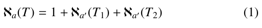where T₁ and T₂ represent the left and right subtree of root, respec- tively.

However, if the root of T is a 1-node, we have

depending on whether s_vl ≥ s_vr or s_vl < s_vr , where v_l and v_r stand for the left and right child of the root.

Now we consider the probability that |T₁| = p and |T₂| = ℵ – p, where ℵ is the number of all nodes in T . This can be estimated by the Bernouli probabilities:

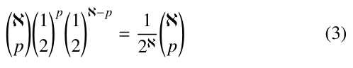
Let c_a,ℵ denote the expected number of nodes created during the execution of PRIORITY-SEARCH( ) against Q. In terms of (1), (2) and (3), we have the following recurrences for ℵ ≥ 2:

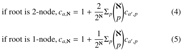
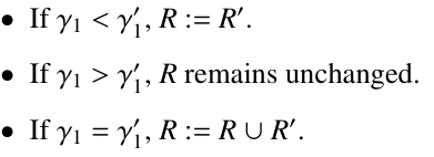
Let γ₁ = 1 if root is a 1-node, and γ₁ = 2 if root is a 2-node.

Then, (4) and (5) can be rewritten as follows:

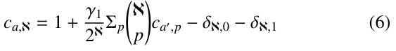
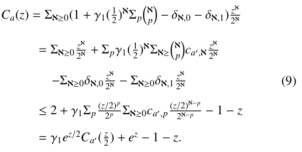
where δ_{ℵ, j} ( j = 0, 1) is equal to 1 if ℵ = j; otherwise, equal to 0. To solve this recursive equation, we consider the following exponential generating function of the average number of nodes searched during the execution of PRIORITY-SEARCH( ).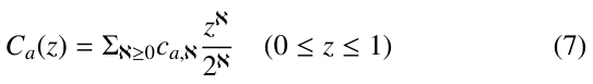

In the following, we will show that the generating function satisfies a relation given below:

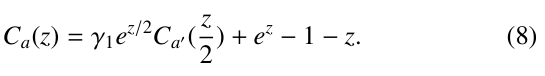
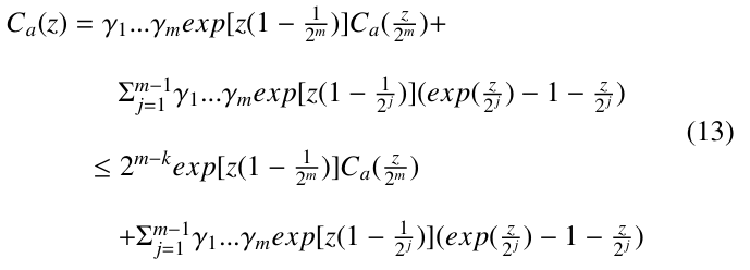
In terms of (6), we rewrite C_a(z) as follows:

Next, we need to compute C_a′ (z), C_a′′ (z), . . . , C_a(m−1) (z). To this end, we define γ_i for i ≥ 2 as follows:

• γ_i = 1, if all the nodes at level i are 1-
• 1 < γ_i ≤ 2, if at least one node at level i is a 2-node. Concretely, γ_i is calculated as below:

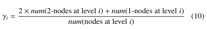
where num(node at level i) represents the number of nodes at level i. In the same way as above, we can get the following equations:

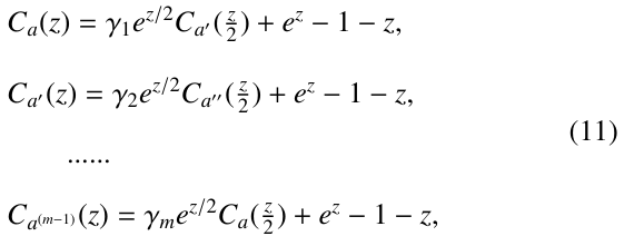
These equations can be solved by successive transportation, as done in [22]. For example, when transporting the expression of C_a′ (z) given by the second equation in (11), we will get

where b(z) = e – 1 – z.

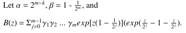
In a next step, we transport C_a′′ into the equation given in (12) Especially, this equation can be successively transformed this way until the relation is only on C_a(z) itself. (Here, we assume that in this process a is circularly shifted.) Doing this, we will eventually get

where k is the number of all those levels each containing only 1- nodes.

We have

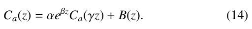
Solving the equation in a way similar to the above, we get

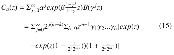
Finally, using the Taylor formula to expand exp(z) and in the above equation, and then extracting the Taylor coefficients, we get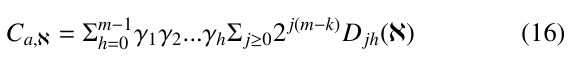

where D₀₀(ℵ) = 1 and for j > 0 or h > 0,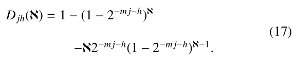

C_a,ℵ can be estimated by using the Mellin transform [23] for summation of series, as done in [22]. According to [22], C_a,ℵ ∼ ℵ^1−k/m. If k/m ≥ 1/2, C_a,ℵ is bounded by O(ℵ^0.5).

It can also be seen that the priority queue can have up to O(2^m/2) nodes on average. Therefore, the running time of extractMax( ) and insert( ) each is bounded by log 2^m/2 = m/2. Thus, the average cost for generating nodes during the process should be bounded by O(mℵ^0.5) ≤ O(m2^m/2). In addition, the whole cost for selecting an attribute to split s_v for each internal node v into its two child nodes: s_vl and s_vr is bounded by O(nm²) since the cost for splitting all the nodes at a level is bounded by O(nm) and the height of T is at most O(m). Here, v_l and v_r represent the left and right child nodes of v, respectively.

So we have the following proposition.

Proposition 2. Let n = |Q| and m be the number of at- tributes in Q. Then, the average time complexity of Algorithm PRIORITY-SEARCH(Q) is bounded by O(nm² + m2^m/2).

4. The Second Algorithm

In this section, we discuss our second algorithm. First, we describe the main idea of this algorithm in Section 4.1. Then, in Section 4.2, we discuss the algorithm in great detail. Next, we analyze the algorithm’s time complexity in Section 4.3.

4.1. Main idea

Let Q = {q₁, …, q_n} be a query log and A = {a₁, …, a_m} be the corresponding set of attributes. For each q_i = c_i1c_i2 . . . c_im (c_{i j} ∈ {0, 1, *}, j = 1, . . . , m), we will create another sequence: r_i = d_j1 … d_jk (k ≤ m), where d_jl = a_jl if c_{i j}l = q_i[ j_l] = 1, or d_jl = (a_jl , *) if c_{i j}l = q_i[ j_l] = * (l ∈ {1, …, k}). If c_{i j}l = q_i[ j_l] = 0, the corresponding a_jl will not appear in r_i at all. Let s and t be the numbers of 1s and *s in q_i, respectively. We can then see that k = s + t.

For example, for q₁ = (1, *, 0, *, 1, *) in Table 1, we will create a sequence shown below:

r₁ = hot-spring. (ride, ∗). (hiking, ∗).airline.(boating, ∗).

Next, we will order all the attributes in Q such that the most fre- quent attribute appears first, but with ties broken arbitrarily. When doing so, (a, *) is counted as an appearance of a. For example, according to the appearance frequencies of attributes in Q (see Table 2), we can define a global ordering for all the attributes in Q as below:

A →Hs→H→B→R→G,

where A stands for airline, Hs for hot spring, H for hiking, B for boating, R for ride, and G for glacier.

Following this general ordering, we can represent each query in Table 1 as a sorted attribute sequense as demonstrated in Table 3 (in this table, the second column shows all the attribute sequences while the third column shows their sorted versions). In the following, by an attribute sequence, we always mean a sorted attribute sequence.

In addition, each sorted query sequence in Table 3 is augmented with a start symbol # and an end symbol $, which are used as sentinels for technical convenience.

Finally, for each query sequence q, we will generate a directed graph G such that each path from the root to a leaf in G represents a package satisfying q. For this purpose, we first discuss a simpler concept.

Definition 4.1. (p-graph) Let q = a₀a₁ … a_ka_k+1 be an attribute sequence representing a query as described above, where a = #, a_k+1 = $, and each a_i (1 ≤ i ≤ k) is an attribute or a pair of the form (a, *); A p-graph over q is a directed graph, in which there is a node for each a_j ( j = 0, …, k + 1); and an edge for (a_j, a_j+1) for each j ∈ {0, …, k}. In addition, there may be an edge from a_j to a_j+2 for each j ∈ {0, …, k – 1} if a_j+1 is a pair (a, *), where a is an attribute.

As an example, consider the p-graph for q₁ = #.A.Hs.(H, *).(B, *).(R, *).$, shown in Fig. 4(a). In this graph, besides a main path going through all the attributes in q₁, we also have three off-line spans, respectively corresponding to three pairs: (H, *), (B, *), and (R, *). Each of them represents an option. For example, going through the span for (H, *) indicates that ‘H’ is not selected while going through ’H’ along the main path indicates that ’H’ is selected.

In the following, we will represent a span by the sub-path (of the main path) covered by it. Then, the above three spans can be represented as follows:

(H, *) – <v₂, v₃, v₄>

(B, *) – <v₃, v₄, v₅>

(R, *) – <v₄, v₅, v₆>.

Here, each sub-path p is simply represented by a set of contigu- ous nodes <v_i1 , …, v_ij > ( j ≥ 3) which p goes through. Then, for the graph shown in Fig. 4, <v₂, v₃, v₄> stands for a sub-path from v₂ to v₄, <v₃, v₄, v₅> for a sub-path from v₃ to v₅, and <v₄, v₅, v₆> for a sub-path from v₄ to v₆.

Table 2: Appearance frequencies of attributes.

attributes	Hs	R	G	H	A	B
appearance frequencies	5/6	6/6	5/6	5/6	5/6	5/6

Table 3: Queries represented as sorted attribute sequences.

query ID	attribute sequences*	sorted attribute sequences
q1	Hs.(R, *).(H, *).A.(B, *).	#.A.Hs.(H, *).(B, *).(R, *).$
q2	Hs.G.(H, *).(A, *).(B, *).	#.(A, *).Hs.(H, *).(B, *).G.$
q3	(Hs, *).H.A.(B, *).	#.A.(Hs, *).H.(B, *).$
q4	(R, *).G.(H, *).A.(B, *).	#.A.(H, *).(B, *).(R, *).G.$
q5	(Hs, *).(H, *).(A, *).	#.(A, *).(Hs, *).(H, *).$
q6	(Hs, *).R.(G, *).(A, *).B.	#.(A, *).(Hs, *).B.R.(G, *).$

*Hs: hot spring, R: ride, G: glacier, H: hiking, A: airline, B: boating.

In fact, what we want is to represent each packages for a query q as a root-to-leaf path in such a graph. However, p-graph fails for this purpose. It is because when we go through from a certain node v to another node u through a span, u must be selected. If u itself represents a (c, *) for some variable name c, the meaning of this ‘*’ is not properly rendered. It is because (c, *) indicates that c is optional, but going through a span from v to (c, *) makes c always selected. So, (c, *) is not well interpreted.

For this reason, we will introduce another concept, the so-called p*-graph, to solve this problem.

Let w₁ = <x₁, …, x_k> and w₂ = <y₁, …, y_l> be two spans in a same p-graph. We say, w₁ and w₂ are overlapped, if one of the two following conditions is satisfied:

• y₁ = x _j for some x _j ∈ {x₂, …, x_k−1}, or
• x₁ = y _j′ for some y _j′ ∈ {y₂, …, y_l−1}

For example, in Fig. 4(a), <v₃, v₄, v₅> (for (B, *)) are over- lapped with both <v₂, v₃, v₄> (for (H, *)) and <v₄, v₅, v₆> (for (R, *)). But <v₂, v₃, v₄> and <v₄, v₅, v₆> are only connected, not overlapped. Being aware of this difference is important since the ovetlapped spans correspond to consecutive *’s while the connected overspans not. More important, the overlapped spans are transitive. That is, if w₁ and w₂ are two overlapped spans, the w₁ ∪ w₂ must be a new, but bigger span. Applying this union operation to all the overlapped spans in a p-graph, we will get their ’transitive closure’. Based on this discussion, we can now define graph G mentioned above.

Definition 4.2. (p*-graph) Let p be the main path in a p-graph P and W be the set of all spans in P. Denote by W* the ’transitive closure’ of W. Then, the p*-graph G with respect to P is defined to be the union of p and W*, denoted as G = p ∪ W*.

See Fig. 4(b) for illustration, in which we show the p*-graph G of the p-graph P shown in Fig. 4(a). From this, we can see that each root-to-leaf path in G represents a package satisfying q₁.

In general, in regard to p*-graphs, we can prove the following important property.

Lemma 1. Let P* be a p*-graph for a query (attribute sequence) q in Q. Then, each path from # to $ in P* represents a package, under which q is satisfied.

Proof. (1) Corresponding to any package σ, under which q is satis- fied, there is definitely a path from # to $. First, we note that under such a package each attribute a_j with q[ j] = 1 must be selected, but with some don’t cares it is selected or not. Especially, we may have more than one consecutive don’t cares that are not selected, which are represented by a span equal to the union of the corre- sponding overlapped spans. Therefore, for σ we must have a path representing it.

(2) Each path from # to $ represents a package, under which q is satisfied. To see this, we observe that each path consists of several edges on the main path and several spans. Especially, any such path must go through every attribute a_j with q[ j] = 1 since for each of them there is no span covering it. But each span stands for a ’*’ or more than one successive ’*’s.

4.2. Algorithm based on trie-like graph search

In this subsection, we discuss how to find a packaget that maxi- mizes the number of satisfied queries in Q. To this end, we will first construct a trie-like structure G over Q, and design a recursive algorithm to search G bottom-up to get results.

Let G₁, G₂, …, G_n be all the p*-graphs constructed for all the queries q_i (i = 1, …, n) in Q, respectively. Denote by p_j and W_j* ( j = 1, …, n) the main path of G _j and the corresponding transitive closure of spans. We will build up G in two steps. In the first step, we will establish a trie, denoted as T = trie(R) over R = {p₁, …, p_n} as follows.

If |R| = 0, trie(R) is, of course, empty. For |R| = 1, trie(R) is a single node. If |R| > 1, R is split into m (possibly empty) subsets R₁, R₂, . . . , R_m so that each R_i (i = 1, . . . , m) contains all those

sequences with the same first attribute name. The tries: trie(R₁), trie(R₂), . . . , trie(R_m) are constructed in the same way except that at the kth step, the splitting of sets is based on the kth attribute (along the global ordering of attributes). They are then connected from their respective roots to a single node to create trie(R).

In Fig. 5(a), we show the trie constructed for the attribute sequences shown in the third column of Table 2. In such a trie, special attention should be paid to all the leaf nodes each labeled with $, representing a query (or a subset of queries). Each edge in the trie is referred to as a tree edge.

The advantage of tries is to cluster common parts of attribute sequences together to avoid possible repeated checking. (Then, this is the main reason why we sort attribute sequences according to their appearance frequencies.) Especially, this idea can also be applied to the attribute subsequences (as will be seen later), over which some dynamical tries can be recursively constructed, leading to an efficient algorithm.

In the following discussion, the attribute c associated with a node v is referred to as the label of v, denoted as l(v) = c.

In addition, we will associate each node v in the trie T with a pair of numbers (pre, post) to speed up recognizing ancestor/descendant relationships of nodes in T , where pre is the order number of v when searching T in preorder and post is the order number of v when searching T in postorder.

These two numbers can be used to check the ancestor/descendant relationships in T as follows.

Let v and v′ be two nodes in T. Then, v′ is a descendant of v iff pre(v′) > pre(v) and post(v′) < post(v).

For the proof of this property of any tree, see Exercise 2.3.2-20 in [24].

For instance, by checking the label associated with v₃ against the label for v₁₂ in Fig. 5(a), we get to know that v₃ is an ancestor of v₁₂ in terms of this property. Particularly, v₃’s label is (3, 9) and v₁₂’s label is (11, 6), and we have 3 < 11 and 9 > 6. We also see that since the pairs associated with v and v do not satisfy this property, v14 must not be an ancestor of v6 and vice versa.
In the second step, we will add all Wi* (i = 1, …, n) to the trie T to construct a trie-like graph G, as illustrated in Fig. 5(b). This trie-like graph is in fact constructed for all the attribute sequences given in Table 2. In this trie-like graph, each span is associated with a set of numbers used to indicate what queries the span belongs to. For example, the span <v2, v3, v4> is associated with three numbers: 3, 5, 6, indicating that the span belongs to 3 queries: q3, q5 and q6. In the same way, the labels for tree edges can also be determined. However, for simplicity, the tree edge labels are not shown in Fig. 5(b).

From Fig. 5(b), we can see that although the number of satisfy- ing packages for queries in Q is exponential, they can be represented by a graph with polynomial numbers of nodes and edges. In fact, in a single p*-graph, the number of edges is bounded by O(n²). Thus, a trie-like graph over m p*-graphs has at most O(n²m) edges.

In a next step, we will search G bottom-up level by level to seek all the possible largest subsets of queries which can be satisfied by a certain package.

First of all, we call a node in T with more than one child a branching node. For instance, node v₁ with two children v₂ and v₁₃ in G shown in Fig. 5(a) is a branching node. For the same reason, v₃, v₄, and v₅ are another three branching nodes.

Node v₀ is not a branching node since it has one child in T (although it has more than one child in G.)

Around the branching node, we have two very important con- cepts defined below.

Definition 4.3. (reachable subsets through spans) Let v be a branching node. Let u be a node on the tree path from root to v in G (not including v itself). A reachable subset of u through spans are all those nodes with a same label c in different subgraphs in G[v] (the subgraph rooted at v) and reachable from u through a span, denoted as RS^v,u[c], where s is a set containing all the labels associated with the corresponding spans.

For RS^v,u[c], node u is called its anchor node.

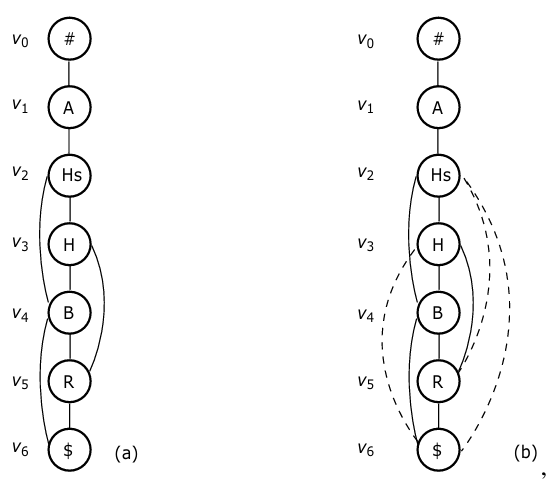
For instance, v₃ in Fig. 5(a) is a branching node (which has two children v₄ and v₁₁ in T ). With respect to v₃, node v₂ on the tree path from root to v₃, has a reachable subset:

We have this RS (reachable subset) due to two spans and  going out of v₂, respectively reaching v₅ and v₈ on two different p*-graphs in G[v₃] with l(v₅) = l(v₁₂) = ‘$’. Then, v₂ is the anchor node of {v₈, v₁₂}.

In general, we are interested only in those RS’s with |RS| ≥ 2 (since any RS with |RS| = 1 only leads us to a leaf node in T and no larger subsets of queries can be found.) So, in the subsequent discussion, by an RS, we always mean an RS with |RS| ≥ 2.

The definition of this concept for a branching node v itself is a little bit different from any other node on the tree path (from root to v). Specifically, each of its RSs is defined to be a subset of nodes reachable from a span or from a tree edge. So for v₃ we have:

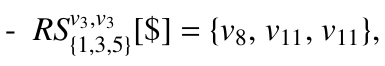
due to two spans , and a tree edge v3 → v12, all going out of v3 with l(v8) = l(v11) = l(v12) = ‘$’. Then, v3 is the anchor node of {v8, v11, v11}.

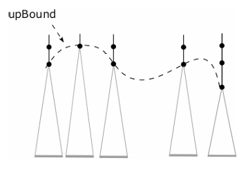
Based on the concept of reachable subsets through spans, we are able to define another more important concept, upper boundaries. This is introduced to recognize all those p*-subgraphs around a branching node, over which a trie-like subgraph needs to be constructed to find some more subsets of queries satisfiable by a certain package.

Definition 4.4.  (upper boundaries) Let v be a branching node. Let v1, v2, …, vk be all the nodes on the tree path from root to v. An upper boundary (denoted as upBounds) with respect to v is a largest subset of nodes {u1, u2, …, uf} with the following properties satisfied:

1. Each u_g (1 ≤ g ≤ f ) appears in some RS_vi[c] (1 ≤ i ≤ k), where c is a label.
2. For any two nodes u_g, u_g′ (g ≠ g^′), they are not related by the ancestor/descendant relationship.

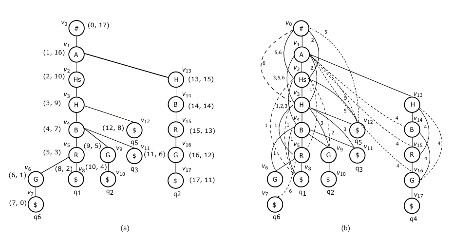
Fig. 6 gives an intuitive illustration of this concept.

As a concrete example, condider branching node v₄ in 5(b). With repect to v₄, we have

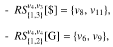
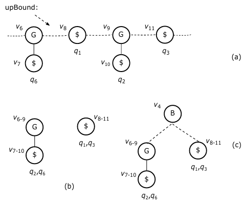
Since all the nodes in these two RSs (v₈, v₆, v₉, and v₁₁) are not related by ancstor/descendant relationsh, they make up an upBound with respect to v₄ (a branching node), as illustrated in 7(a).

Then, we will construct a trie-like graph over all the four p*- subgraphs, each starting from a node on the upBound. See Fig. 7(b) for illustration, where v₆₋₉ stands for the merging v₆ and v₉, v₇₋₁₀ for the merging v₇ and v₁₀, and v₈₋₁₁ for the merging v₈ and v₁₁.

Obviously, this can be done by a recursive call of the algorithm itself.

In addition, for technical convenience, we will add the corre- sponding branching node (v₄) to the trie as a virtual root, and v₄ → v₆₋₉ and v₃ → v₈₋₁₁ as two virtual edges, each associated with the corresponding RSs to facilitate the search of all those packages satisfying corresponding queries. This is because to find such packages we need to travel through this branching node to the root of T . See Fig. 9(c) for illustration.

Specifically, the following operations will be carried out when encountering a branching node v.

• Calculate all RSs with respect v.
• Calculate the upBound in terms of RS
• Make a recursive call of the algorithm over all the subgraphs within G[v] each rooted at a node on the corresponding up-

In terms of the above discussion, we design a recursive algo- rithm to do the task, in which R is used to accommodate the result, represented as a set of triplets of the form:

<α, β, γ>,

where α stands for a subset of conjunctions, β for a truth assignment satisfying the conjunctions in α, and γ is the size of α. Initially, R = ∅.

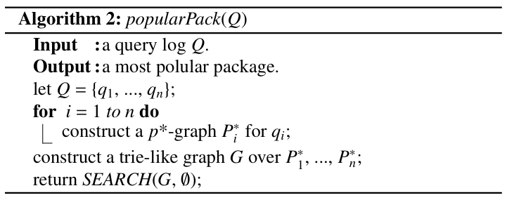
The input of popularPack( ) is a query log Q = {q₁, …, q_n}. First, we will build up a p*-graph for each q_i (i = 1, …, n), over which a trie-like graph G will be constructed (see lines 2 – 4). Then, we call a recursive algorithm SEARCH( ) to produce the result (see line 5), which is a set of triplets of the form <α, β, γ> with the same largest γ value. Thus, each β is a popular package.

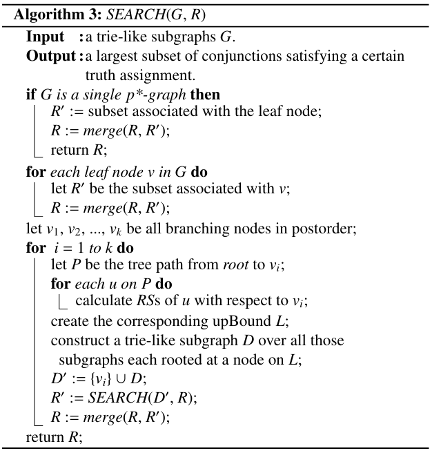
SEARCH( ) works recurcively. Its input is a pair: a trie-like subgraph G^′ and a set R^′ of triplets <α, β, γ> found up to now. Initially, G^′ = G and R = ∅.

First, we check whether G is a single p*-graph. If it is the case, we must have found a largest subset of queries associated with the leaf node, satisfiable by a certain package. This subset should be merged into R (see lines 1 – 4).

Otherwise, we will search G bottom up to find all the branching nodes in G. But before that, each subset of queries associated with a leaf node in R will be first merged into R (see line 5 – 7).

For each branching node v encountered, we will check all the nodes u on the tree path from root to v and compute their RSs (reach- able subsets through spans, see lines 8 – 12), based on which we then compute the corresponding upBound with respect to v (see line 13). According to the upBound L, a trie-like graph D will be created over a set of subgraphs each rooted at a node on L (see line 14). Next, v will be added to D as its root (see line 15). Here, we notice that D^′ := {v} ∪ D is a simplified representation of an operation, by which we add not only v, but also the corresponding edges to D. Next, a recursive call of the algorithm is made over D^′ (see linee 16). Finally, the result of the recursive call of the algorithm will be merged into the global answer (see line 17).

Here, the merge operation used in line 3, 7, 17 is defined as below.

Let R = {r1, …, rt} for some t ≥ 0 with each ri = <αi, βi, γi>.
We have γ1 = γ2 =… = γt. Let for some s ≥ 0 with each We have By merge(R, R′), we will do the following checks. 

In the above algorithm, how to figure out β in a triple <α, β, γ> is not specified. For this, however, some more operations should be performed. Specifically, we need to trace each chain of recursive calls of SEARCH( ) for this task.

Let SEARCH(G₀, R₀) → SEARCH(G₁, R₁) → … SEARCH(G_k, R_k) be a consecutive recursive call process during the execution of SEARCH( ), where G₀ = G, R₀ = ∅, and G_i is a trie-like subgraph constructed around a branching node in G_i−1 and R_i is the result obtained just before SEARCH(G_i, R_i) is invoked (i = 1, …, k).

Assume that during the execution of SEARCH(G_k, R_k) no further recursive call is conducted. Then, R_k can be a single p*-graph, or a trie-like subgraph, for which no RS RS ¿ 1 for any branching node can be found. Denote by r _j the root of G_j and by v _j the branching node around which SEARCH(G_j+1, R_j+1) is invoked ( j = 0, …, k – 1). Denote by T _j the trie in G_j.

Then, the labels on all the paths from r _j in T _j for j ∈ {1, … k} (connected by using the corresponding anchor nodes) consist of β in the corresponding triple <α, β, γ> with α being a subset of queries associated with a leaf node in G_k. As an example, consider the the trie-like subfraph G^′ shown in Fig. 7(c) again. In the execution, we will have a chains of recursive calls as below.

SEARCH(G, …) → SEARCH(G^′, …)

Along this chain, we will find two query subset Q1 = {q2, q6} (associated with leaf node v7−10) and Q2 = {q1, q3} (associated with leaf node v7−10). To find the package for Q1, we will trace the path in G′ bottom from v7−10 to v6−10, the reverse edge (recognized according to [G]), and then the path from v4 → to v0
in G. Since {1, 2} does not contain 6, q6 should be removed from Q1. The package is {A, Hs, H, B, G}. In the same way, we can find the package {A, Hs, H, B} for Q2 = {q1, q3}.

The following example helps for illustrating the whole working process.

Example 2. When applying SEARCH( ) to the p*-graphs con- structed for all the attribute sequences given in Table 1, we will first construct a trie-like graph G shown in Fig. 5(b). Searching G bottom up, we will encounter four branching nodes: v₅, v₄, v₃ and v₁.

For each branching node, a recursive call of SEARCH( ) will be carried out. But we show here only the recursive call around v₁ for simplicity. With respect to v₁, we have only one RS with |RS| > 1:

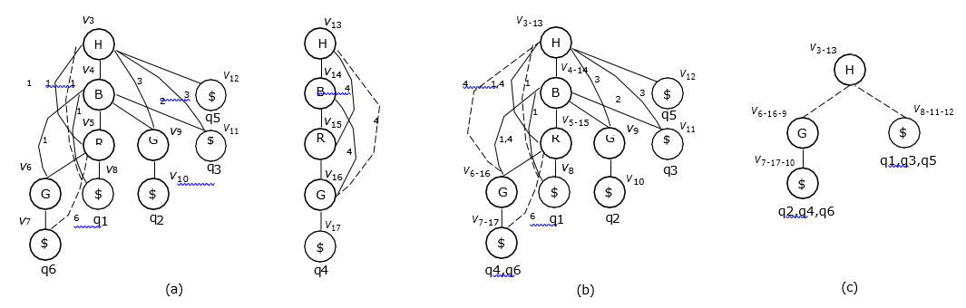
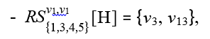
Due to span  and tree edge v₁→ v₁₃.

Therefore, the corresponding upBound is {v₃, v₁₃}. Then, a new trie-like subgraphs (see Fig. 8(b)) will be constructed by merging two subgraphs shown in Fig. 8(a).

In Fig. 8(b), the node v₃₋₁₃ represents a merging of two nodes v₃ and v₁₃ in Fig. 8(a). All the other merging nodes v₄₋₁₄, v₅₋₁₅, v₆₋₁₆, and v₇₋₁₇ are created in the same way.

When applying SEARCH( ) to this new trie-like subgraph, we will check all its branching nodes v₅₋₁₅, v₄₋₁₄, and v₃₋₁₃ in turn. Especially, with respect to v₃₋₁₃, we have

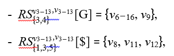
According to these RSs, we will contruct a trie-like subgraph as shown in Fig. 8(c). From this subgraph, we can find another two query subsets {q₂, q₄, q₆} and {q₁, q₃, q₅}, respectively satisfiable by two packages {A, H, G} and {A, Hs, H}.

In the execution of SEARCH( ), much redundancy may be con- ducted, but can be easily removed. See Fig. 9(a) for illustration.

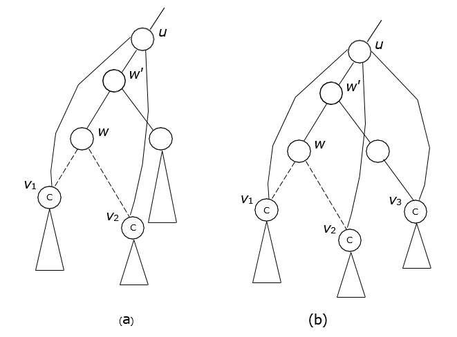
In this figure, w and w^′ are two branching nodes. With respect to w and w^′, node u will have the same RSs. That is, we have

RS^w,u[C] = RS^w′,u[C] = {v , v }.

Then, in the execution of SEARCH( ), the corresponding trie- like subgraph will be created two times, but with the same result produced.

However, this kind of redundancy can be simply removed in two ways.

In the first method, we can examine, by each recursive call, whether the input subgraph has been checked before. If it is the case, the corresponding recursive call will be suppressed.

In the second method, we create RSs only for those nodes appear- ing on the segment (on a tree path) between the current branching node and the lowest ancestor branching node in T . In this way, we may lose some answers. But the most popular package can always be found. See Fig. 9(b) for illustration. In this case, the RS of u with respect to w is different from the RS with respect to w^′. However, when we check the branching node w, will not be computed and therefore the corresponding result will not be generated. But must cover  . Therefore, a package satisfying a larger, or a same-sized subset of queries will definitely be found.

4.3. Time complexity analysis

The total running time of the algorithm consists of three parts.

The first part, denoted as τ_‘, is the time for computing the fren- quencies of attribute appearances in Q. Since in this process each attribut in a q_i is accessed only once, τ₁ = O(nm).

The second part, denoted as τ₂, is the time for constructing a trie-like graph G for Q. This part of time can be further partitioned into three portions.

• τ₂₁: The time for sorting attribute sequences for q_i’s. It is obviously bounded by O(nmlog₂ m).
• τ₂₂: The time for constructing p*-graphs for each q_i (i = 1,…, n). Since for each variable sequence a transitive closure over its spans should be first created and needs O(m²) time, this part of cost is bounded by O(nm²).
• τ₂₃: The time for merging all p*-graphs to form a trie-like graph G, which is also bounded by O(nm²).

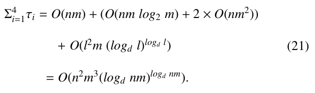
The third part, denoted as τ₃, is the time for searching G to find a maximum subset of conjunctions satisfied by a certain truth assignment. It is a recursive procedure. To analyze its running time, therefore, a recursive equation should established. Let l = nm. Assume that the average outdegree of a node in T is d. Then the average time complexity of τ₄ can be characterized by the following recurrence: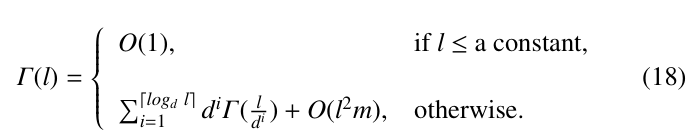

Here, in the above recursive equation, O(l²m) is the cost for generating all the reachable subsets of a node through spans and upper boundries, together with the cost for generating local trie-like subgraphs for each recursive call of the algorithm. We notice that the size of all the RSs together is bounded by the number of spans in G, which is O(lm).

From (4), we can get the following inequality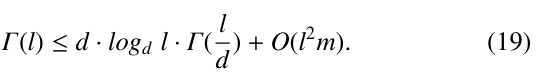

Solving this inequality, we will get

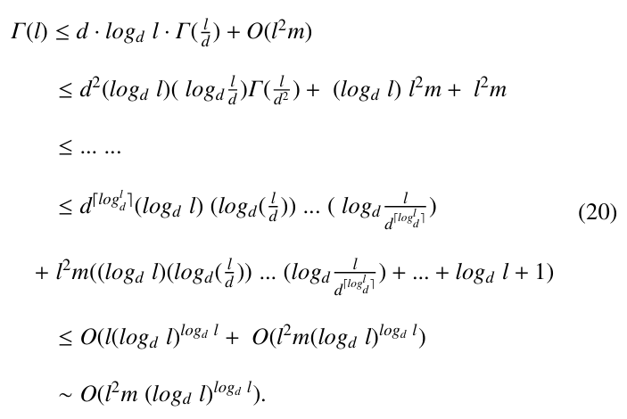
Thus, the value for τ₃ is Γ(l) ∼ O(l²m (log_d l)^logd l).

From the above analysis, we have the following proposition.

Proposition 3. The average running time of our algorithm is bounded by

But we remark that if the average outdegree of a node in T is < 2, we can use a brute-force method to find the answer in poly- nomial time. Hence, we claim that the worst case time complexity is bounded by O(l²m(log₂ l)^log2 l) since (log_d l)^logd l decreases as d increases.

5. Conclusions

In this paper, we have discussed two new method to solve the problem to find a most popular package in terms of a given questionnaire. The first method is based on a kind of tree search, but with the pri- ority queue structure being utilized to control the tree exploration. Together with a powerful heuristics, this approach enables us to cut off a lot of futile branches and find an answer as early as possible in the tree search process. The average time complexity is bounded by O(nm² + m2^m/2), where n = |Q| and m is the number of attributes in the query log |Q|. The main idea behind the second method is to construct a graph structure, called p*-graph. In this way, all the bottom up, we can find the answer efficiently. the average time complexity of the algorithm is bounded by O(n²m³(log₂ nm)^log2 nm).

As a future work, we will make a detailed analysis of the impact of the heuristics discussed in Section 4.2 to avoid any repeated recursive calls. If it is the case, the number of recursive calls for each branching node will be bounded by O(m) since the height of the trie-like graph G is bounded by O(m). Thus, the worst-case time complexity of our algorithm should be bounded by O(n²m⁴). It is because we have at most O(nm) branching nodes, and for each recursive call we need O(nm²) time to construct a dynamical trie. So, the total running time will be O(nm) × O(m) × O(nm²) = O(n²m⁴).

Conflict of Interest  The authors declare no conflict of interest.

1. [1] R. Agrawal, T. Imieli´nski, A. Swami, “Mining association rules between sets of items in large databases,” in Proceedings of the 1993 ACM SIGMOD International Conference on Management of Data, 207–216, Association for Computing Machinery, 1993, doi:10.1145/170035.170072.
2. B. Gavish, D. Horsky, K. Srikanth, “An Approach to the Optimal Positioning of a New Product,” Management Science, 29, 1277–1297, 1983, doi:10.1287/mnsc.29.11.1277.
3. T. S. Gruca, B. R. Klemz, “Optimal new product positioning: A genetic algorithm approach,” European Journal of Operational Research, 146, 621–633, 2003, doi:https://doi.org/10.1016/S0377-2217(02)00349-1.
4. J. Resig, A. Teredesai, “A framework for mining instant messaging services,” in In Proceedings of the 2004 SIAM DM Conference, 2004.
5. J. Han, J. Pei, Y. Yin, “Mining frequent patterns without candidate generation,” SIGMOD Rec., 29, 1–12, 2000, doi:10.1145/335191.335372.
6. M. Miah, G. Das, V. Hristidis, H. Mannila, “Standing Out in a Crowd: Selecting Attributes for Maximum Visibility,” in 2008 IEEE 24th International Conference on Data Engineering, 356–365, 2008, doi:10.1109/ICDE.2008.4497444.
7. J. C.-W. Lin, Y. Li, P. Fournier-Viger, Y. Djenouri, L. S.-L. Wang, “Mining High-Utility Sequential Patterns from Big Datasets,” in 2019 IEEE International Conference on Big Data (Big Data), 2674–2680, 2019, doi:10.1109/BigData47090.2019.9005996.
8. A. Tonon, F. Vandin, “gRosSo: mining statistically robust patterns from a sequence of datasets,” Knowledge and Information Systems, 64, 2329–2359, 2022, doi:10.1007/s10115-022-01689-2.
9. Y. Chen, W. Shi, “On the Designing of Popular Packages,” in 2018 IEEE International Conference on Internet of Things (iThings) and IEEE Green Computing and Communications (GreenCom) and IEEE Cyber, Physical and Social Computing (CPSCom) and IEEE Smart Data (SmartData), 937–944, 2018, doi:10.1109/Cybermatics 2018.2018.00180.
10. M. Miah, “Most popular package design,” in 4th Conference on Information Systems Applied Research, 2011.
11. R. Kohli, R. Krishnamurti, P. Mirchandani, “The Minimum Satisfiability Problem,” SIAM Journal on Discrete Mathematics, 7, 275–283, 1994, doi:10.1137/S0895480191220836.
12. S. A. Cook, The Complexity of Theorem-Proving Procedures, 143–152, Association for Computing Machinery, 1st edition, 2023.
13. Y. Chen, “Signature files and signature trees,” Information Processing Letters, 82, 213–221, 2002, doi:https://doi.org/10.1016/S0020-0190(01)00266-6.
14. Y. Chen, “On the signature trees and balanced signature trees,” in 21st International Conference on Data Engineering (ICDE’05), 742–753, 2005, doi:10.1109/ICDE.2005.99.
15. Y. Chen, Y. Chen, “On the Signature Tree Construction and Analysis,” IEEE Transactions on Knowledge and Data Engineering, 18, 1207–1224, 2006, doi:10.1109/TKDE.2006.146.
16. F. Grandi, P. Tiberio, P. Zezula, “Frame-sliced partitioned parallel signature files,” in Proceedings of the 15th Annual International ACM SIGIR Conference on Research and Development in Information Retrieval, 286–287, Association for Computing Machinery, 1992, doi:10.1145/133160.133211.
17. D. L. Lee, Y. M. Kim, G. Patel, “Efficient signature file methods for text retrieval,” IEEE Transactions on Knowledge and Data Engineering, 7, 423–435, 1995, doi:10.1109/69.390248.
18. D. L. Lee, C.-W. Leng, “Partitioned signature files: design issues and performance evaluation,” ACM Trans. Inf. Syst., 7, 158–180, 1989,
    doi:10.1145/65935.65937.
19. Z. Lin, C. Faloutsos, “Frame-sliced signature files,” IEEE Transactions on Knowledge and Data Engineering, 4, 281–289, 1992, doi:10.1109/69.142018.
20. E. Tousidou, P. Bozanis, Y. Manolopoulos, “Signature-based structures for objects with set-valued attributes,” Information Systems, 27, 93–121, 2002, doi:https://doi.org/10.1016/S0306-4379(01)00047-3.
21. T. H. Cormen, C. E. Leiserson, R. L. Rivest, C. Stein, Introduction to algorithms, MIT press, 2022.
22. P. Flajolet, C. Puech, “Partial match retrieval of multidimensional data,” J. ACM, 33, 371–407, 1986, doi:10.1145/5383.5453.
23. L. Debnath, D. Bhatta, Integral transforms and their applications, Chapman and Hall/CRC, 2016.
24. E. K. Donald, “The art of computer programming,” Sorting and searching, 3, 4, 1999.

This paper is currently not cited.

No. of Downloads Per Month

No. of Downloads Per Country