Hybrid Optical Scanning Holography for Automatic Three-Dimensional Reconstruction of Brain Tumors from MRI using Active Contours
Volume 9, Issue 4, Page No 07-13, 2024
Author’s Name: Abdennacer El-Ouarzadi1, Anass Cherkaoui1, Abdelaziz Essadike2, Abdenbi Bouzid1
View Affiliations
1 Moulay Ismail University, Physical Sciences and Engineering, Faculty of Sciences, Meknès, 11201, Morocco
2Hassan First University of Settat, Higher Institute of Health Sciences, Laboratory of Health Sciences and Technologies, Settat, 26000, Morocco
a)whom correspondence should be addressed. E-mail: a.elouarzadi@edu.umi.ac.ma
Adv. Sci. Technol. Eng. Syst. J. 9(4), 07-13 (2024); ![]() DOI: 10.25046/aj090402
DOI: 10.25046/aj090402
Keywords: Bain tumor detection, Fully Automatic Segmentation, Active contour, Optical Scanning Holography (OSH), 3D Automatic Reconstruction

Export Citations
This paper presents a method for automatic 3D segmentation of brain tumors in MRI using optical scanning holography. Automatic segmentation of tumors from 2D slices (coronal, sagittal and axial) enables efficient 3D reconstruction of the region of interest, eliminating the human errors of manual methods. The method uses enhanced optical scanning holography with a cylindrical lens, scanning line by line, and displays MRI images via a spatial light modulator. The outgoing phase component of the scanned data, collected digitally, reliably indicates the position of the tumor.The tumor position is fed into an active contour model (ACM), which speeds up segmentation of the seeding region. The tumor is then reconstructed in 3D from the segmented regions in each slice, enabling tumor volume to be calculated and cancer progression to be estimated. Experiments carried out on patient MRI datasets show satisfactory results. The proposed approach can be integrated into a computer-aided diagnosis (CAD) system, helping doctors to localize the tumor, estimate its volume and provide 3D information to improve treatment techniques such as radiosurgery, stereotactic surgery or chemotherapy administration. In short, this method offers a precise and reliable solution for the segmentation and 3D reconstruction of brain tumors, facilitating diagnosis and treatment.
Received: 03 May 2024, Revised: 26 June 2024, Accepted: 27 June 2024, Published Online: 10 July 2024
1. Introduction
A brain tumor is a mass of abnormal cells involved in a chaotic process of somatic driver mutations [1,2], where they cause various symptoms and increase the risk of brain damage. In fact, the secondary tumor infiltrates neighboring healthy tissues and proliferates within the brain or its membranes, making it critical to determine its shape and volume to ensure effective management of patients in the early stages of cancer. Magnetic resonance imaging (MRI) is the most commonly used non-invasive imaging modality for brain tumor detection [3–5]. MRI uses radio waves and a strong magnetic field to create a series of cross-sectional images of the brain. In other words, the 3D anatomical details of a tumor are represented as a set of parallel 2D cross-sectional images. Representing 3D data as projected 2D slices results in a loss of information and can raise questions about tumor prognosis. In addition, 2D slices do not accurately represent the complexity of brain anatomy. Therefore, interpretation of 2D images requires specialized training. Therefore, volume reconstruction from sequential parallel 2D cross-sectional slices is a necessity for 3D tumor visualization, In 2013, the authors in [6] proposed an improved interpolation technique to estimate missing slices and the Marching Cubes (MC) algorithm to mesh the tumor. For surface rendering, they applied the Phong shading and lighting model to better compute the tumor volume.
The 3D reconstruction of tumors first requires an appropriate segmentation of the region of interest. This 3D reconstruction helps radiologists to better diagnose patients and subsequently remove the entire tumor when surgical intervention is considered. Techniques presented in [7,8] are based on preprocessing, image enhancement, and contouring prior to reconstruction. In 2012, authors in [9] used a technique based on phase-contrast projection tomography to calculate the 3D density distribution in bacterial cells. In addition, an approach proposed by [10] in 2019 provides a technique for segmenting brain tumors in the 3D volume using a 2D convolutional neural network for tumor prediction. Authors in [11,12] conducted a comparison between conventional machine learning based techniques and deep learning based techniques. The latter are further categorized into 2D CNN and 3D CNN techniques. However, the results of techniques based on deep convolutional neural networks out perform those of machine learning techniques. As for the authors in [13,14], they introduced a two-stage optimal mass transport technique (TSOMT), which involve stransforming an irregular 3D brain image into a cube with minimal deformation, for segmenting 3D medical images. Automatic segmentation of a brain tumor from two-dimensional slices (coronal, sagittal, and axial), facilitated by convolutional neural networks [15], significantly aids in delineating the region of interest in 3D.
Conventional holography was invented by [16] in 1948 during his research to improve the resolution of electron microscopes. This invention evolved in the 1960s with the advent of lasers, and holograms were recorded on plates or photosensitive films based primarily on silver ions that darkened under the influence of light. With the progress of high-resolution matrix detectors, digital holography was generalized in 1994 by the authors in [17], paving the way for numerous applications: holographic microscopy [18–20], quantitative phase imaging [21–23], color holography [24–26], metrology [27–29], holographic cameras [30], 3D displays [31–34], and head-up displays [35,36]. Authors in [37] were the first to use phase-shifting holography to eliminate unwanted diffraction orders from the hologram. They introduced spatial phase shifting using a piezoelectric transducer with a mounted mirror [38], and slight frequency modifications of acousto-optic modulators (AOMs) [39–41]. The latter technique is closely related to heterodyne detection methods.
Optical Scanning Holography (OSH) is considered an intelligent application for processing the pupil interaction. The pupil interaction scheme was implemented using optical heterodyne scanning by Korpel and Poon in 1979, and the use of an interaction scheme in a scanning illumination mode was developed by Indebetouw and Poon in 1992. By modifying one of the twolenses relative to the other (specifically, one lensis an open mask and the other is a pinhole mask) and defocusing the optical system, in 1985 author in [42] developed an optical scanning system capable of holographically recording a scanned object. This technique led to the invention of optical scanning holography. OSH has various applications, including optical scanning microscopy, 3D shape recognition, 3D holographic TV, 3D optical remote sensing, and more.
Early work on preprocessing in the OSH system dates back to 1985. Later, it was shown that placing a Gaussian annular aperture instead of a flat lens is useful for recovering the edge of a cross-sectional image in a hologram [43,44]. In 2010, authors in [45] demonstrated that by choosing a pupil function such as the Laplacian of the Gaussian, the performance of the method is an efficient means to extract the edge of a 3D scanned object by the OSH system. The authors in [46] proposed a 1D image acquisition system for auto stereoscopic display consisting of a cylindrical lens, a focusing lens, and an imaging device. By scanning an object over a wide angle, the synthesized image can beviewed as a 3D stereoscopic image.
The aim of this paper is to propose and develop a fully automatic 3D segmentation of brain tumors from magnetic resonance images. The proposed model is based on the same principle as our previous articles [47,48] and specifically for the segmentation of high and low grade glioblastoma brain tumors. To achieve this goal, the following contributions are made:
- Proposing a fully automated 3D method for brain tumor segmentation from MRI image sequences.
- Improving the conventional optical scanning holography technique by exploiting the properties of the cylindrical lens to optimize the scanning process and shorten the holographic recording process.
- Transitioning active contour theory from semi-automatic to fully automatic status with reliable tumor detection.
- Perform tests to demonstrate the effectiveness of our method using the well-known BraTS 2019 and BraTS 2020 databases.
2. Materials And Methods
2.1. Data used
The database of brain tumor images used in this study was obtained from the Medical Image Computing and Computer Assisted Intervention (MICCAI) 2019 and MICCAI 2020 Multimodal Brain Tumor Segmentation Challenges, organized in collaboration with B. Menze, A. Jakab, S. Bauer, M. Reyes, M. Prastawa, and K. Van Leemput. It includes 40 glioma patients, including 20 high-grade (HG) and 20 low-grade (LG) cases, with four MRI sequences (T1, T1C, T2, and FLAIR) available for each patient. The challenge data base contains fully anonymized images collected from the ETH Zurich, the University of Debrecen, the University of Bern, and the University of Utah. All images are linearly co-registered and craniocaudally oriented. Institutional review board approval was not required as all human subject data are publicly available and de-identified [1,3].
2.2. Methodology
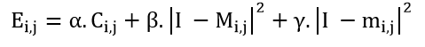
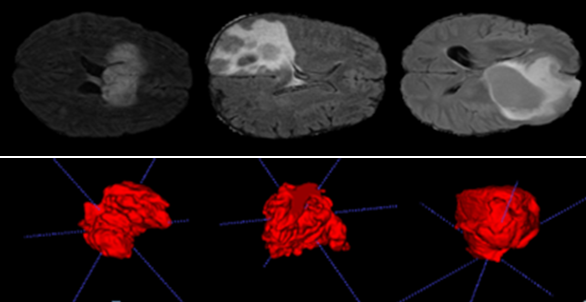
Figure 1 shows the optical scanning holography system used in our method. A laser beam of frequency ω isshifted in frequency to ψ and ψ+Δψ by Acousto-Optic Modulators (AOM) 1 and 2, respectively. The beams from the AOMs are then collimated by collimators BE1 and BE2. The out going beam from BE2 is considered as a plane wave of frequency ω+ψ+Δψ, which is projected onto the object by the x-y scanner. Our novel method involves the integration of a cylindrical lens L1 into the chosen imaging system, which provides a cylindrical wave at ω+Ω that is projected onto the object. A focusing lens is also used to capture a large number of elementary images containing extensive parallax data. These elemental images are transformed into a matrix of elemental images, where each captured elemental image corresponds to a vertical line in ray space [46]. Using this linear scanning technique, object images are captured in a single pass rather than point-by-point, and the shape of the surface is adjusted after each iteration, saving computational time. Accordingly, after appropriate sampling for viewing conditions, we achieved fully automatic segmentation through the improved algorithm and arrangement of color filters. This allowed the transformation of two-dimensional element images into Three-Dimensional (3D) images, as shown in Figures 5 and 6.
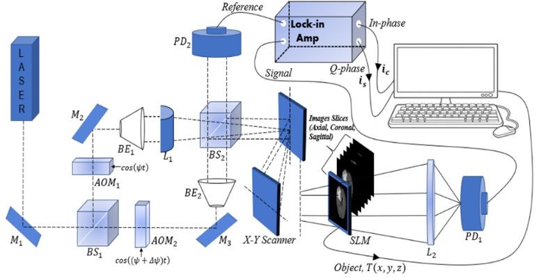
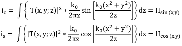
The x-y scanner is used to scan the 3D object uniformly, line by line. As a result, each scan line of the object corresponds to a line in the hologram at the same vertical position. Along each scan line, Photo-Detectors PD1 and PD2 are used to capture the optical signal scattered by the object and the heterodyne frequency information ∆Ω as a reference signal, respectively, and convert them into electrical signals for the lock-in amplifier. The in-phase and quadrature-phase outputs of the lock-in amplifier circuit produce a sine hologram, H_sin (x, y), and a cosine hologram, H_cos (x, y), to achieve a complete 2D scan of the object, as shown below:
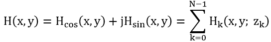
with:
2.3. Detection
Tumor contours are typically identified by fast pixel transitions, which indicate a significant change in information, while slow variations are eliminated by differentiation. Several methods are used for contour detection, including derivative methods based on evaluating the variation at each pixel by searching for maxima using a gradient or Laplacian filter.
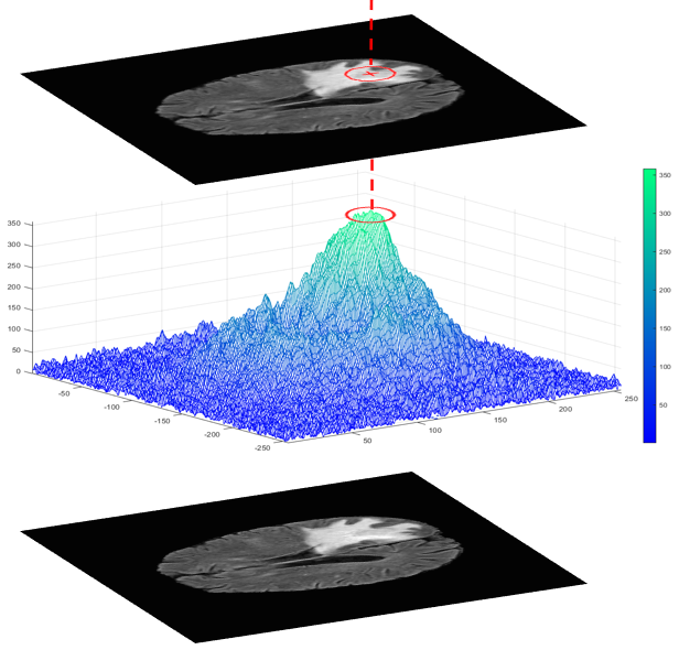
The optical system in Figure 1 provides an output showing the distribution of both the phase and quadrature component of the heterodyne current. We will focus only on the phase component to extract the phase current after scanning the object images line by line. The maximum values characterizing this output are referred to as the peaks of the phase component.
Figure 2 illustrates how the initial contour C(i, j) is extracted from the peaks of the phase component maxima obtained from the optical scanning holography (OSH), i.e., the maximum of the intensity ic with:
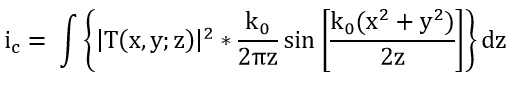
Contours delineating these maxima are drawn, resulting in regions that designate the position of the tumor within the tumor tissue.
The output results of the Optical Scanning Holography(OSH) optical process are implemented numerically to extract the following parameters:
- C: the center of the tumor.
- L: the amplitude of the peak of the phase component.
- Ci: the initial contour formed using the principle illustrated in Figure 2.
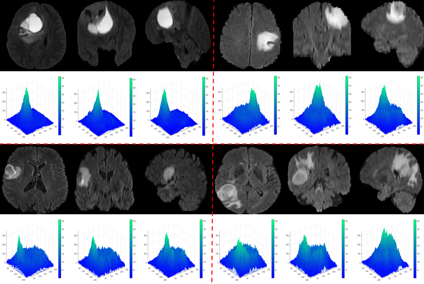
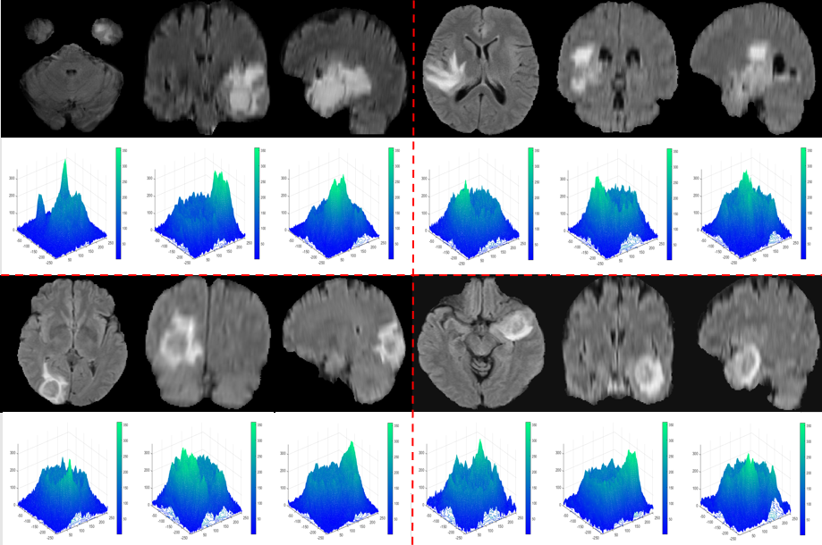
Figures 3 and 4 provide examples of phase component peaks obtained using the OSH method.
2.4. Segmentation and 3D Reconstruction
The segmentation of brain tumors using the active contour approach has received increasing attention. In this article, a fully automated active contour approach based on the OSH technique is proposed. This approach requires significant computational time. However, this technique allows a contour to be iteratively deformed to divide an image into several meaningful regions. Whitaker was able to reduce the computational time in his efficient Sparse Field Method algorithm by accurately representing the target surface. In this method, each point of the target surface is processed, compared with the initialization curve, and updated after each iteration.
The novelty of our research is to apply the OSH technique by integrating a cylindrical lens into our system to improve the detection phase in terms of precision and acquisition time by processing the image of the region of interest line by line (line-by-line scanning).
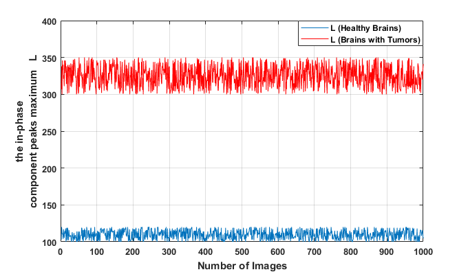
It is true that the calculation of the terms of the active contour energy, as shown below, has allowed us to achieve an exact and precise segmentation of brain tumors. However, this segmentation is conditioned by the choice of an initial contour Ci,j, which gives it a semi-automatic nature :
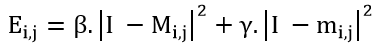
In our work, we have proposed a model of active contours combined with the OSH approach, which enables us to address the issue of manual supervision in selecting the initial contour, especially for complex tumor shapes. We have achieved, through the use of the maximum phase current of the OSH, which corresponds to the initial contour of the active contour model, an improvement in the detection of tumor tissue contours. By adding the term derivedfrom the OSH technique, we were able to automate our model :
This article builds upon previous work in the field of 3D reconstruction, primarily by combining it with enhanced detection and segmentation techniques. Indeed, this new technique improves the computational efficiency and precision in selecting the pixels that are crucial for reconstructing 3D object shapes.
The results of reconstructing 3D object images from a real patient dataset are presented in Figures 5 and 6.
3. Experimental Results
3.1. evaluation of detection phase
To extract brain tumors accurately, it is essential to reliably determine the parameter L (where L represents the maximum peak of the phase component). That’s why we studied the values of L on different MRI images from Brats-2018 and Brats-2019 containing tumor tissues.
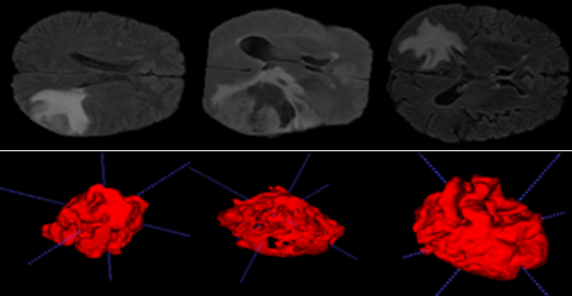
We observe that the values of L in the case of tumors are significantly separated from those of healthy brain tissue. We also notice that all the maxima of the phase components provided by the OSH process, used for tumor detection, fall within the range [300;350], while for healthy tissue, they are in the interval [100;150].
3.2. Evaluation of segmentation phase
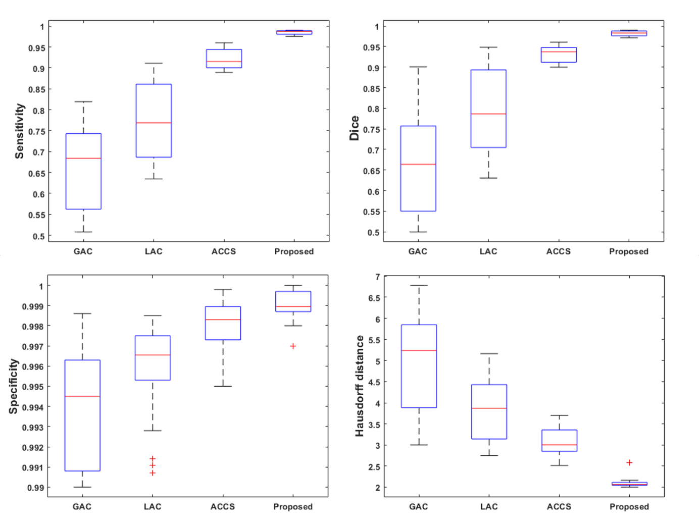
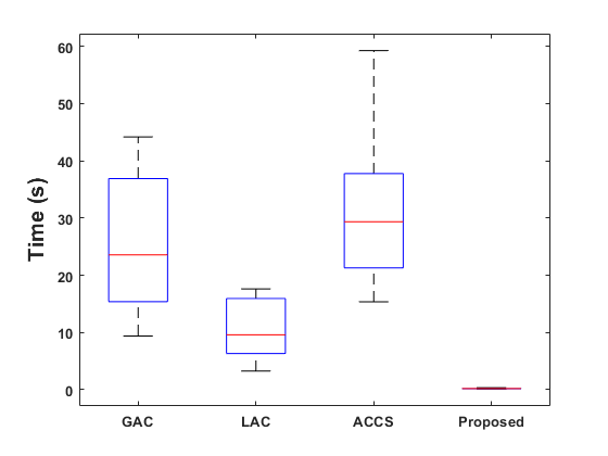
Figure 8 displays box plots for the sensitivity, Dice score, specificity, and Hausdorff distance obtained by our method on the Brats-2019 and Brats-2020 datasets. The performance of our method is compared to that of the Geodesic Active Contour (GAC) model, Localized Active Contour (LAC), and Cuckoo-driven Active Contour (ACCS) models. We note that the performance of the proposed methodis the most satisfactory in terms of segmentation versus the other methods compared, particularly in terms of sensitivity, specificity and Dice score. The statistical computation time of the most relevant steps of our algorithm per MRI image is given in figure 9.
3.3. Evaluation of reconstruction phase
The data in tables (1 and 2) enable us to obtain the tumor volume for each patient with very respectable accuracy, making it easier to estimate the degree of cancer. These tables also provide useful information such as brain volume and mean intensity for each patient label (brain label and tumor label).
Table 1: 3-D Segmentation results of real patient data from the BRATS 2019 database.
| Patients | Labels | Voxel count | Volume (mm3) | Intensity Mean ±SD |
| Patient 1 | Clear Label | 8 812 673 | 8.812673 x10⁶ | 32.4629 ± 76.7841 |
| Label with tumor | 115 327 | 1.15327 x10⁵ | 434.7898 ± 75.9586 | |
| Patient 2 | Clear Label | 8 908 742 | 8.908742 x10⁶ | 31.0648 ± 66.3003 |
| Label with tumor | 19 258 | 1.9258 x10⁴ | 424.8549 ± 65.4917 | |
| Patient 3 | Clear Label | 8 896 112 | 8.896112 x10⁶ | 24.4006 ± 649036 |
| Label with tumor | 31 888 | 3.1888 x10⁴ | 451.9312 ± 57.2040 | |
| Patient 4 | Clear Label | 8 893 509 | 8.893509 x10⁶ | 36.5984 ± 90.5500 |
| Label with tumor | 34 491 | 3.4491 x10⁴ | 1137.5650 ± 202.0132 | |
| Patient 5 | Clear Label | 8 874 450 | 8.874450 x10⁶ | 34.4983 ± 78.4227 |
| Label with tumor | 53 550 | 5.3550 x10⁴ | 432.8664 ± 75.4400 | |
| Patient 6 | Clear Label | 8 815 463 | 8.815463 x10⁶ | 31.0447 ± 74.2778 |
| Label with tumor | 112 537 | 1.12537 x10⁵ | 451.1814 ± 65.6239 | |
| Patient 7 | Clear Label | 8 800 705 | 8.800705 x10⁶ | 21.7560 ± 56.5531 |
| Label with tumor | 127 295 | 1.27295 x10⁵ | 305.4569 ± 57.3601 | |
| Patient 8 | Clear Label | 8 872 783 | 8.872783 x10⁶ | 29.3676 ± 68.4357 |
| Label with tumor | 55 217 | 5.5217 x10⁴ | 334.1023 ± 48.2186 | |
| Patient 9 | Clear Label | 8 920 644 | 8.920644 x10⁶ | 11.8151 ± 32.1527 |
| Label with tumor | 7 356 | 7.356 x10³ | 198.0174 ± 38.5634 | |
| Patient 10 | Clear Label | 8 911 678 | 8.911678 x10⁶ | 23.9592 ± 59.2099 |
| Label with tumor | 16 322 | 1.6322 x10⁴ | 454.6847 ± 83.4070 | |
| Patient 11 | Clear Label | 8 900 834 | 8.900834 x10⁶ | 35.1428 ± 75.6676 |
| Label with tumor | 27 166 | 2.7166 x10⁴ | 344.4761 ± 46.2303 | |
| Patient 12 | Clear Label | 8 833 615 | 8.833615 x10⁶ | 64.3847 ± 39.4228 |
| Label with tumor | 94 385 | 9.4385 x10⁴ | 580.9401 ± 36.3711 | |
| Patient 13 | Clear Label | 8 876 743 | 8.876743 x10⁶ | 68.8470 ± 153.2978 |
| Label with tumor | 51 257 | 5.1257 x10⁴ | 698.3368 ± 120.9774 | |
| Patient 14 | Clear Label | 8 698 867 | 8.698867 x10⁶ | 25.9308 ± 57.5036 |
| Label with tumor | 229 131 | 2.29131 x10⁵ | 304.6895 ± 70.7478 | |
| Patient 15 | Clear Label | 8 778 460 | 8.778460 x10⁶ | 44.1679 ± 112.9932 |
| Label with tumor | 149 540 | 1.49540 x10⁵ | 442.8497 ± 45.4427 | |
| Patient 16 | Clear Label | 8 801 474 | 8.801474 x10⁶ | 18.6908 ± 43.6618 |
| Label with tumor | 126 526 | 1.26526 x10⁵ | 241.1445 ± 36.7579 | |
| Patient 17 | Clear Label | 8 690 176 | 8.690176 x10⁶ | 16.6104 ± 39.7039 |
| Label with tumor | 237 824 | 2.37824 x10⁵ | 213.0597 ± 45.3580 | |
| Patient 18 | Clear Label | 8 833 752 | 8.833852 x10⁶ | 16.8981 ± 43.7038 |
| Label with tumor | 94 248 | 9.8248 x10⁴ | 270.6864 ± 44.3378 | |
| Patient 19 | Clear Label | 8 699 808 | 8.699808 x10⁶ | 16.7930 ± 41.8654 |
| Label with tumor | 228 192 | 2.28192 x10⁵ | 227.5470 ± 37.6771 | |
| Patient 20 | Clear Label | 8 902 965 | 8.902965 x10⁶ | 47.3972 ± 115.0547 |
| Label with tumor | 25 035 | 2.5035 x10⁴ | 477.4638 ± 28.0403 |
Table 2: 3-D Segmentation results of real patient data from the BRATS 2020 database.
| Patients | Labels | Voxel count | Volume (mm3) | Intensity Mean ±SD |
| Patient 1 | Clear Label | 8796585 | 8.796585 x10⁶ | 32.0395 ± 76.2065 |
| Label with tumor | 131415 | 1.31415 x10⁵ | 413.8778 ± 90.8952 | |
| Patient 2 | Clear Label | 8899672 | 8.899672 x10⁶ | 30.7910 ± 65.7704 |
| Label with tumor | 28328 | 2.8328 x10⁴ | 384.8039 ± 81.0838 | |
| Patient 3 | Clear Label | 8880808 | 8.880808 x10⁶ | 25.9012 ± 63.8240 |
| Label with tumor | 47192 | 4.7192 x10⁴ | 4079188 ± 80.5098 | |
| Patient 4 | Clear Label | 8875910 | 8.875910 x10⁶ | 35.4049 ± 86.3327 |
| Label with tumor | 52090 | 5.2090 x10⁴ | 968.9609 ± 299.9311 | |
| Patient 5 | Clear Label | 8863102 | 8.863102 x10⁶ | 34.2085 ± 78.1643 |
| Label with tumor | 64898 | 6.4898 x10⁴ | 402.7914 ± 81.2011 | |
| Patient 6 | Clear Label | 8794503 | 8.794503 x10⁶ | 30.4320 ± 73.2910 |
| Label with tumor | 133497 | 1.33497 x10⁵ | 425.5790 ± 84.9031 | |
| Patient 7 | Clear Label | 8828307 | 8.828307 x10⁶ | 22.3986 ± 57.6266 |
| Label with tumor | 99693 | 9.9693 x10⁴ | 327.0939 ± 44.3143 | |
| Patient 8 | Clear Label | 8777055 | 8.777055 x10⁶ | 21.3723 ± 53.5396 |
| Label with tumor | 150945 | 1.50945 x10⁵ | 347.9547 ± 73.5984 | |
| Patient 9 | Clear Label | 8859507 | 8.859507 x10⁶ | 29.0185 ± 67.8758 |
| Label with tumor | 68493 | 6.8493 x10⁴ | 320.2008 ± 54.0278 | |
| Patient 10 | Clear Label | 8856743 | 8.856743 x10⁶ | 30.1615 ± 71.5588 |
| Label with tumor | 71257 | 7.1257 x10⁴ | 410.5989 ± 110.6990 | |
| Patient 11 | Clear Label | 8852777 | 8.852777 x10⁶ | 41.6819 ± 100.7240 |
| Label with tumor | 75223 | 7.5223 x10⁴ | 568 0779 ± 103.8634 | |
| Patient 12 | Clear Label | 8825129 | 8.825129 x10⁶ | 70.7885 ± 174.1385 |
| Label with tumor | 102871 | 1.02871 x10⁵ | 761.5829 ± 89.2313 | |
| Patient 13 | Clear Label | 8811475 | 8.811475 x10⁶ | 19.5354 ± 43.5697 |
| Label with tumor | 116525 | 1.16525 x10⁵ | 226.5449 ± 29.4236 | |
| Patient 14 | Clear Label | 8829255 | 8.829255 x10⁶ | 17.1114 ± 39.8459 |
| Label with tumor | 98745 | 9.8745 x10⁴ | 223.5896 ± 27.5731 | |
| Patient 15 | Clear Label | 8907363 | 8.907363 x10⁶ | 41.1899 ± 100.3383 |
| Label with tumor | 20637 | 2.0637 x10⁴ | 405..570 ± 35.2389 | |
| Patient 16 | Clear Label | 8781794 | 8.781794 x10⁶ | 19.6149 ± 45.3264 |
| Label with tumor | 146206 | 1.46206 x10⁵ | 243.5090 ± 39.3731 | |
| Patient 17 | Clear Label | 8852596 | 8.852596 x10⁶ | 17.1913 ± 45.4955 |
| Label with tumor | 75404 | 7.5404 x10⁴ | 279.9906 ± 49.1193 | |
| Patient 18 | Clear Label | 8831696 | 8.831696 x10⁶ | 37.5604 ± 103.4473 |
| Label with tumor | 96304 | 9.6304 x10⁴ | 390.8695 ± 40.2213 | |
| Patient 19 | Clear Label | 8823355 | 8.823355 x10⁶ | 75.8865 ± 180.9212 |
| Label with tumor | 104645 | 1.04645 x10⁵ | 649.1030 ± 55.8957 | |
| Patient 20 | Clear Label | 8829763 | 8.829763 x10⁶ | 9.3929 ± 32.4282 |
| Label with tumor | 98237 | 9.8237 x10⁴ | 229.8103 ± 44.2263 |
5. Conclusion
The aim of this article is to develop a 3D reconstruction and quantification approach to facilitate physician surgical planning and tumor volume calculation. The three-dimensional model of the brain tumor was reconstructed from a given set of two-dimensional brain slices (axial, coronal, and sagittal). In the slices containing tumors, the improved Optical Scanning Holography (OSH) method helped us to extract the maximum component in phase, and at the same time an Active Contour Model (ACM) was applied to this area of interest to perform a faster segmentation of the region corresponding to the tumors in each slice. We obtained satisfactory results with different active contour models with different similarity parameters on database images (BRATS 2019 and 2020), compared to several state-of-the-art brain tumor segmentation methods.
The application of this method does, however, present a number of limitations. Firstly, integration with existing diagnostic and processing systems can pose challenges, particularly with regard to the compatibility of data formats and communication protocols. In addition, the quality and resolution of MRI images are crucial to the success of the method. Low-quality images can result in imprecise segmentation and inaccurate 3D reconstruction, compromising the accuracy and clinical utility of the method. Therefore, high-quality images and resolution of integration issues are essential to maximize the effectiveness of this approach in a clinical setting.
To improve this method, it is necessary to validate its efficacy more widely and robustly in a variety of clinical settings. In the future, it will be necessary to refine the technology for greater accuracy, improve the quality of MRI images, and ensure seamless integration with other tools for diagnosing and treating brain tumors by resolving data compatibility issues. These efforts will open up new prospects for research and innovation in this field.
Conflict of Interest
All authors disclose any financial and personal relationships with other people or organizations that could inappropriately influence our work.
The authors declare no conflict of interest.
Acknowledgment
Authors thank Raphael Meier, University of Bern, Medical Image Analysis Institute for Surgical Technology and Biomechanics Switzerland, for securing available access to the Multimodal Brain Tumor Segmentation Benchmark (BRATS).
- T.J. Hudson, “The International Cancer Genome Consortium,” Cancer Research, 176(1), 139–148, 2009, doi:10.1038/nature08987.International.
- S. Bakas, H. Akbari, A. Sotiras, M. Bilello, M. Rozycki, J.S. Kirby, J.B. Freymann, K. Farahani, C. Davatzikos, “Advancing The Cancer Genome Atlas glioma MRI collections with expert segmentation labels and radiomic features,” Scientific Data, 4(1), 170117, 2017, doi:10.1038/sdata.2017.117.
- R. Ranjbarzadeh, A. Bagherian Kasgari, S. Jafarzadeh Ghoushchi, S. Anari, M. Naseri, M. Bendechache, “Brain tumor segmentation based on deep learning and an attention mechanism using MRI multi-modalities brain images,” Scientific Reports, 11(1), 10930, 2021, doi:10.1038/s41598-021-90428-8.
- R.P.J., “BRAIN TUMOR MRI IMAGE SEGMENTATION AND DETECTION IN IMAGE PROCESSING,” International Journal of Research in Engineering and Technology, 03(13), 1–5, 2014, doi:10.15623/ijret.2014.0313001.
- B.H. Menze, A. Jakab, S. Bauer, J. Kalpathy-Cramer, K. Farahani, J. Kirby, Y. Burren, N. Porz, J. Slotboom, R. Wiest, L. Lanczi, E. Gerstner, M.-A. Weber, T. Arbel, B.B. Avants, N. Ayache, P. Buendia, D.L. Collins, N. Cordier, J.J. Corso, A. Criminisi, T. Das, H. Delingette, C. Demiralp, C.R. Durst, M. Dojat, S. Doyle, J. Festa, F. Forbes, et al., “The Multimodal Brain Tumor Image Segmentation Benchmark (BRATS),” IEEE Transactions on Medical Imaging, 34(10), 1993–2024, 2015, doi:10.1109/TMI.2014.2377694.
- The Efficiency of 3D-Printed Dog Brain Ventricular Models from 3 Tesla (3T) Magnetic Resonance Imaging (MRI) for Neuroanatomy Education, The Pakistan Veterinary Journal, 2024, doi:10.29261/pakvetj/2024.168.
- M. Bartels, M. Priebe, R.N. Wilke, S.P. Krüger, K. Giewekemeyer, S. Kalbfleisch, C. Olendrowitz, M. Sprung, T. Salditt, “Low-dose three-dimensional hard x-ray imaging of bacterial cells,” Optical Nanoscopy, 1(1), 10, 2012, doi:10.1186/2192-2853-1-10.
- K. Pawar, Z. Chen, N. Jon Shah, G.F. Egan, An Ensemble of 2D Convolutional Neural Network for 3D Brain Tumor Segmentation, 359–367, 2020, doi:10.1007/978-3-030-46640-4_34.
- M. kamal Al-anni, P. DRAP, “Efficient 3D Instance Segmentation for Archaeological Sites Using 2D Object Detection and Tracking,” International Journal of Computing and Digital Systems, 15(1), 1333–1342, 2024, doi:10.12785/ijcds/150194.
- G. Gunasekaran, M. Venkatesan, “An Efficient Technique for Three-Dimensional Image Visualization Through Two-Dimensional Images for Medical Data,” Journal of Intelligent Systems, 29(1), 100–109, 2019, doi:10.1515/jisys-2017-0315.
- H. Khan, S.F. Alam Zaidi, A. Safi, S. Ud Din, A Comprehensive Analysis of MRI Based Brain Tumor Segmentation Using Conventional and Deep Learning Methods, 92–104, 2020, doi:10.1007/978-3-030-43364-2_9.
- V. Kumar, T. Lal, P. Dhuliya, D. Pant, “A study and comparison of different image segmentation algorithms,” in 2016 2nd International Conference on Advances in Computing, Communication, & Automation (ICACCA) (Fall), IEEE: 1–6, 2016, doi:10.1109/ICACCAF.2016.7749007.
- M. Eliasof, A. Sharf, E. Treister, “Multimodal 3D Shape Reconstruction under Calibration Uncertainty Using Parametric Level Set Methods,” SIAM Journal on Imaging Sciences, 13(1), 265–290, 2020, doi:10.1137/19M1257895.
- W.-W. Lin, C. Juang, M.-H. Yueh, T.-M. Huang, T. Li, S. Wang, S.-T. Yau, “3D brain tumor segmentation using a two-stage optimal mass transport algorithm,” Scientific Reports, 11(1), 14686, 2021, doi:10.1038/s41598-021-94071-1.
- P. Li, W. Wu, L. Liu, F. Michael Serry, J. Wang, H. Han, “Automatic brain tumor segmentation from Multiparametric MRI based on cascaded 3D U-Net and 3D U-Net++,” Biomedical Signal Processing and Control, 78, 103979, 2022, doi:10.1016/j.bspc.2022.103979.
- D. GABOR, “A New Microscopic Principle,” Nature, 161(4098), 777–778, 1948, doi:10.1038/161777a0.
- U. Schnars, W. Jüptner, “Direct recording of holograms by a CCD target and numerical reconstruction,” Applied Optics, 33(2), 179, 1994, doi:10.1364/AO.33.000179.
- W. Xu, M.H. Jericho, I.A. Meinertzhagen, H.J. Kreuzer, “Digital in-line holography for biological applications,” Proceedings of the National Academy of Sciences, 98(20), 11301–11305, 2001, doi:10.1073/pnas.191361398.
- P. Marquet, B. Rappaz, P.J. Magistretti, E. Cuche, Y. Emery, T. Colomb, C. Depeursinge, “Digital holographic microscopy: a noninvasive contrast imaging technique allowing quantitative visualization of living cells with subwavelength axial accuracy,” Optics Letters, 30(5), 468, 2005, doi:10.1364/OL.30.000468.
- J. Garcia-Sucerquia, W. Xu, S.K. Jericho, P. Klages, M.H. Jericho, H.J. Kreuzer, “Digital in-line holographic microscopy,” Applied Optics, 45(5), 836, 2006, doi:10.1364/AO.45.000836.
- E. Cuche, F. Bevilacqua, C. Depeursinge, “Digital holography for quantitative phase-contrast imaging,” Optics Letters, 24(5), 291, 1999, doi:10.1364/OL.24.000291.
- B. Rappaz, P. Marquet, E. Cuche, Y. Emery, C. Depeursinge, P.J. Magistretti, “Measurement of the integral refractive index and dynamic cell morphometry of living cells with digital holographic microscopy,” Optics Express, 13(23), 9361, 2005, doi:10.1364/OPEX.13.009361.
- B. Kemper, G. von Bally, “Digital holographic microscopy for live cell applications and technical inspection,” Applied Optics, 47(4), A52, 2008, doi:10.1364/AO.47.000A52.
- N. Demoli, D. Vukicevic, M. Torzynski, “Dynamic digital holographic interferometry with three wavelengths,” Optics Express, 11(7), 767, 2003, doi:10.1364/OE.11.000767.
- J. Zhao, H. Jiang, J. Di, “Recording and reconstruction of a color holographic image by using digital lensless Fourier transform holography,” Optics Express, 16(4), 2514, 2008, doi:10.1364/OE.16.002514.
- P. Tankam, P. Picart, D. Mounier, J.M. Desse, J. Li, “Method of digital holographic recording and reconstruction using a stacked color image sensor,” Applied Optics, 49(3), 320, 2010, doi:10.1364/AO.49.000320.
- F. Charrière, J. Kühn, T. Colomb, F. Montfort, E. Cuche, Y. Emery, K. Weible, P. Marquet, C. Depeursinge, “Characterization of microlenses by digital holographic microscopy,” Applied Optics, 45(5), 829, 2006, doi:10.1364/AO.45.000829.
- J.-M. Desse, P. Picart, P. Tankam, “Digital three-color holographic interferometry for flow analysis,” Optics Express, 16(8), 5471, 2008, doi:10.1364/OE.16.005471.
- P. Tankam, Q. Song, M. Karray, J. Li, J. Michel Desse, P. Picart, “Real-time three-sensitivity measurements based on three-color digital Fresnel holographic interferometry,” Optics Letters, 35(12), 2055, 2010, doi:10.1364/OL.35.002055.
- K. Kim, H. Yoon, M. Diez-Silva, M. Dao, R.R. Dasari, Y. Park, “High-resolution three-dimensional imaging of red blood cells parasitized by Plasmodium falciparum and in situ hemozoin crystals using optical diffraction tomography,” Journal of Biomedical Optics, 19(01), 1, 2013, doi:10.1117/1.JBO.19.1.011005.
- F. Yaraş, H. Kang, L. Onural, “Real-time phase-only color holographic video display system using LED illumination,” Applied Optics, 48(34), H48, 2009, doi:10.1364/AO.48.000H48.
- P.-A. Blanche, A. Bablumian, R. Voorakaranam, C. Christenson, W. Lin, T. Gu, D. Flores, P. Wang, W.-Y. Hsieh, M. Kathaperumal, B. Rachwal, O. Siddiqui, J. Thomas, R.A. Norwood, M. Yamamoto, N. Peyghambarian, “Holographic three-dimensional telepresence using large-area photorefractive polymer,” Nature, 468(7320), 80–83, 2010, doi:10.1038/nature09521.
- J. Geng, “Three-dimensional display technologies,” Advances in Optics and Photonics, 5(4), 456, 2013, doi:10.1364/AOP.5.000456.
- M. Kujawinska, T. Kozacki, C. Falldorf, T. Meeser, B.M. Hennelly, P. Garbat, W. Zaperty, M. Niemelä, G. Finke, M. Kowiel, T. Naughton, “Multiwavefront digital holographic television,” Optics Express, 22(3), 2324, 2014, doi:10.1364/OE.22.002324.
- H. Mukawa, K. Akutsu, I. Matsumura, S. Nakano, T. Yoshida, M. Kuwahara, K. Aiki, M. Ogawa, “8.4: Distinguished Paper : A Full Color Eyewear Display Using Holographic Planar Waveguides,” SID Symposium Digest of Technical Papers, 39(1), 89–92, 2008, doi:10.1889/1.3069819.
- C. Jang, C.-K. Lee, J. Jeong, G. Li, S. Lee, J. Yeom, K. Hong, B. Lee, “Recent progress in see-through three-dimensional displays using holographic optical elements [Invited],” Applied Optics, 55(3), A71, 2016, doi:10.1364/AO.55.000A71.
- I. Yamaguchi, Phase-Shifting Digital Holography, Springer US: 145–171, 2006, doi:10.1007/0-387-31397-4_5.
- I. Yamaguchi, J. Kato, S. Ohta, J. Mizuno, “Image formation in phase-shifting digital holography and applications to microscopy,” Applied Optics, 40(34), 6177, 2001, doi:10.1364/AO.40.006177.
- F. Le Clerc, L. Collot, M. Gross, “Numerical heterodyne holography with two-dimensional photodetector arrays,” Optics Letters, 25(10), 716, 2000, doi:10.1364/OL.25.000716.
- E. Absil, G. Tessier, M. Gross, M. Atlan, N. Warnasooriya, S. Suck, M. Coppey-Moisan, D. Fournier, “Photothermal heterodyne holography of gold nanoparticles,” Optics Express, 18(2), 780, 2010, doi:10.1364/OE.18.000780.
- B. Samson, F. Verpillat, M. Gross, M. Atlan, “Video-rate laser Doppler vibrometry by heterodyne holography,” Optics Letters, 36(8), 1449, 2011, doi:10.1364/OL.36.001449.
- T.-C. Poon, Three-dimensional image processing and optical scanning holography, 329–350, 2003, doi:10.1016/S1076-5670(03)80018-6.
- Y. Zhang, R. Wang, P. Tsang, T.-C. Poon, “Sectioning with edge extraction in optical incoherent imaging processing,” OSA Continuum, 3(4), 698, 2020, doi:10.1364/OSAC.383473.
- G. Indebetouw, W. Zhong, D. Chamberlin-Long, “Point-spread function synthesis in scanning holographic microscopy,” Journal of the Optical Society of America A, 23(7), 1708, 2006, doi:10.1364/JOSAA.23.001708.
- X. Zhang, E.Y. Lam, “Edge detection of three-dimensional objects by manipulating pupil functions in an optical scanning holography system,” in 2010 IEEE International Conference on Image Processing, IEEE: 3661–3664, 2010, doi:10.1109/ICIP.2010.5652483.
- Y. Momonoi, K. Taira, Y. Hirayama, “Scan-type image capturing system using a cylindrical lens for one-dimensional integral imaging,” in: Woods, A. J., Dodgson, N. A., Merritt, J. O., Bolas, M. T., and McDowall, I. E., eds., in Stereoscopic Displays and Virtual Reality Systems XIV, 649017, 2007, doi:10.1117/12.703170.
- A. Cherkaoui, A. El-Ouarzadi, A. Essadike, Y. Achaoui, A. Bouzid, “Brain Tumor Detection and Segmentation Using a Hybrid Optical Method by Active Contour,” in 2023 International Conference on Digital Age & Technological Advances for Sustainable Development (ICDATA), IEEE: 132–138, 2023, doi:10.1109/ICDATA58816.2023.00032.
- A. EL-OUARZADI, A. Cherkaoui, A. Essadike, A. Bouzid, “Brain Tumor Detection and Segmentation Using a Hybrid Optical Method by Active Contour,” Available at SSRN 4629062, doi:10.2139/ssrn.4629062.
No. of Downloads Per Month