Solar Photovoltaic Power Output Forecasting using Deep Learning Models: A Case Study of Zagtouli PV Power Plant
Volume 9, Issue 3, Page No 41-48, 2024
Author’s Name: Sami Florent Palm1,a), Sianou Ezéckie Houénafa², Zourkalaïni Boubakar³, Sebastian Waita¹, Thomas Nyachoti Nyangonda¹, Ahmed Chebak4
View Affiliations
¹Condensed Matter Research Group, Department of Physics, University of Nairobi, Nairobi, Kenya
²Institute for Basic Science, Technology and Innovation, Pan African University, Nairobi, Kenya
³Ecole Doctorale Informatique, Télécommunication et Electronique, Sorbonne Université, Paris, France
4Green Tech Institute, Mohammed VI Polytechnic University, Benguerir, Morocco
a)whom correspondence should be addressed. E-mail: palm@students.uonbi.ac.ke
Adv. Sci. Technol. Eng. Syst. J. 9(3), 41-48(2024); ![]() DOI: 10.25046/aj090304
DOI: 10.25046/aj090304
Keywords: Deep learning, LSTM, GRU, Solar PV Power, Zagtouli

Export Citations
Forecasting solar PV power output holds significant importance in the realm of energy management, particularly due to the intermittent nature of solar irradiation. Currently, most forecasting studies employ statistical methods. However, deep learning models have the potential for better forecasting. This study utilises Long Short-Term Memory (LSTM), Gate Recurrent Unit (GRU) and hybrid LSTM-GRU deep learning techniques to analyse, train, validate, and test data from the Zagtouli Solar Photovoltaic (PV) plant located in Ouagadougou (longitude:12.30702o and latitude:1.63548o), Burkina Faso. The study involved three evaluation metrics: Root Mean Square Error (RMSE), Mean Absolute Error (MAE), and coefficient of determination (R2). The RMSE evaluation criteria gave 10.799(LSTM), 11.695(GRU) and 10.629(LSTM-GRU) giving the LSTM-GRU model as the best for RMSE evaluation. The MAE evaluation provided 2.09, 2.1 and 2.0 for the LSTM, GRU and LSTM-GRU models respectively, showing that the LSTM-GRU model is superior for MAE evaluation. The R2 criteria similarly showed the LSTM-GRU model to be best with 0.999 compared to 0.998 for LSTM and 0.997 for GRU. It becomes evident that the hybrid LSTM-GRU model exhibits superior predictive capabilities compared to the other two models. These results indicate that the hybrid LSTM-GRU model has the potential to reliably predict the solar PV power output. It is therefore recommended that the authorities in charge of the solar PV Plant in Ouagadougou should consider switching to the deep learning LSTM-GRU model.
Received: 22 March 2024, Revised: 6 May 2024, Accepted: 7 May 2024, Published Online: 25 May 2024
1. Introduction
In the pursuit of sustainable and renewable energy sources, solar photovoltaic (PV) systems have emerged as a leading solution for harnessing the abundant energy provided by the sun. A critical factor in optimizing the efficiency and reliability of solar PV installations is the accurate forecasting of power output [1,2]. This is particularly vital for ensuring the seamless integration of solar energy into the existing power grid and effectively managing energy resources.
The application of deep learning techniques has gained considerable attention in this context due to its capacity to model complex relationships within large datasets, offering a promising tool to enhance the precision of solar PV power output forecasting [3].
Researchers in [4] employed techniques to improve the performance of grid-connected PV systems. Financial and technical limitations emerge as hindrances to the development of PV systems, prompting a recommendation for the utilization of artificial intelligence to enhance power generation. Comparison between time series methods and artificial intelligence-based methods for power output prediction in a large grid-connected PV plant in China indicated the efficiency of neural network models over statistical models for PV power output prediction, particularly for short-term forecasts [5]. In a solar power prediction study in India, the efficiency of Long Short-Term Memory (LSTM) and Backpropagation Neural Network (BPNN) models was compared, confirming the effectiveness of the LSTM model [3]. LSTM and Multi-layer Perception (MLP) techniques were employed to forecast short-term solar PV power. A comparison of their performance based on parameters like Mean Absolute Errors (MAE), Mean Absolute Percentage Error (MAPE), Root Mean Square Error (RMSE), and R2 revealed LSTM as the superior model [6]. A hybrid deep learning model for short-term PV power forecasting, integrating Wavelet Packet Decomposition (WPD) and LSTM, exhibits remarkable accuracy and stability. However, additional investigation is needed for long-term forecasting, especially during cloudy and rainy periods [7]. A method is proposed that combines LSTM-RNN and temporal correlation principles for PV power prediction, showcasing enhanced predictive capabilities and emphasizing the interplay between climate and electricity production [8]. The hybrid model (VMD-ISSA-GRU), integrating Variational Mode Decomposition (VMD), Improved Sparrow Search Algorithm (ISSA), and GRU, was utilized to improve PV power prediction. Results showed strong performance with an MAE of 1.0128 kW, RMSE of 1.5511 kW, and R-squared value of 0.9993 [9]. The study in [10] presents a new forecasting method for a large grid- connected PV plant in Vietnam, emphasizing climate uncertainty and employing the LSTM algorithm. The result underscored the impact of climate data on prediction accuracy, emphasizing the need for careful model configuration. The study suggests the importance of using LSTM configurations tailored to specific climatic and operational conditions. PV power generation, inherently linked to unpredictable weather conditions, poses challenges in prediction. The case studies presented reflect the ongoing efforts to develop more accurate forecasting methods to address the intermittency and instability of PV systems connected to the power grid. As per the existing literature, the LSTM model proves highly proficient in forecasting solar PV power. Moreover, its amalgamation with other models demonstrates superior effectiveness compared to the individual performance of each model.
Limited literature has been undertaken in Burkina Faso and Sahel countries in general regarding the forecasting of solar PV power using deep learning methods. This study underscores the necessity of advanced forecasting techniques using LSTM, GRU and hybrid LSTM-GRU models in predicting the output of the Zagtouli PV power. Forecasting in Zagtouli is important since more energy is needed to meet regional power demands. By delving into the challenges associated with traditional forecasting methods, the study aims to contribute valuable insights to the broader field of renewable energy research, paving the way for improved efficiency and reliability in the integration of solar power. The findings hold the potential to deepen our understanding of the dynamics influencing solar energy production and inform future developments in sustainable energy planning and management. The remainder of this paper will be structured as follows: first, the methodology, followed by the results and discussions, and finally, the conclusion and perspectives.
2. Methodology
2.1. Zagtouli PV Power Plant
The Zagtouli Solar PV Power Plant sits in Ouagadougou, the capital of Burkina Faso, positioned at a longitude of 12.30702o and latitude -1.63548o. Figure 1 depicts the location of the Zagtouli PV facility in Burkina Faso. This PV Plant has a total installed capacity of 33.696 MWp composed of 16 subsystems. In this study, one subsystem of 2.3 MW is considered.

2.2. Deep Learning Models
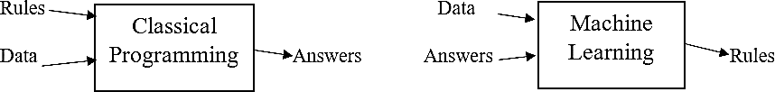
In brief, Artificial Intelligence (AI) is the endeavour to automate cognitive tasks typically executed by humans [11]. Consequently, AI constitutes a broad domain that encompasses not only Machine Learning (ML) and Deep Learning (DL) but also various other approaches that may not necessitate any form of learning [12].ML is the art of studying algorithms that learn from examples and experiences [13]. The difference from hardcoding is that the machine learns on its own to find such rules [13]. Figure 2 below shows the difference between classical programming and ML.
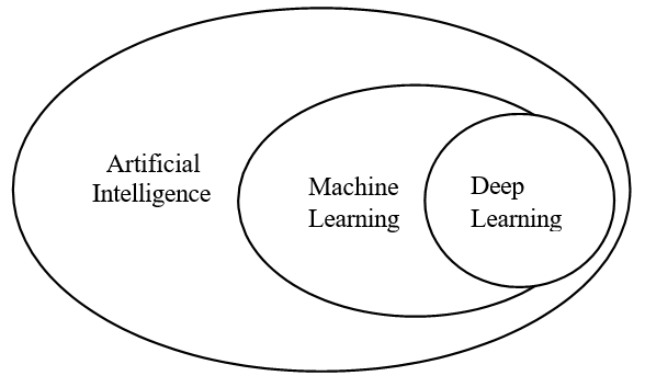
Deep Learning (DL), a subset of Machine Learning (ML), represents a novel approach to deriving meaningful representations from data by prioritizing the acquisition of progressively more meaningful representations across successive layers [12]. Figure 3 explains the difference between AI, ML and DL.
The DL technique is fundamentally based on the Artificial Neuron Network (ANN) which is ML method known as the artificial intelligence system which reflects the human brain. To comprehend the fundamental structure of ANN, it is essential to first grasp the concept of a ‘node.’ The general configuration of a node is depicted in Figure 4 below:
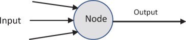
Every node receives an array of inputs through connections and transmits them to neighbouring nodes [14]. Figure 5 depicts the overall model of an ANN, inspired by the functioning of a biological neuron [15]. Nodes are organized into linear networks referred to as layers. The ANN comprises three layers: the input layer, the output layer, and the hidden layer [16]. In the input layer, X1, X2, X3, … Xn represent multiple inputs to the network. Meanwhile, W1, W2, W3, … Wn are referred to as connection weights, indicating the strength associated with a specific node. In ANN, weights are regarded as crucial factors since they are numerical parameters that influence the interactions among neurons, playing a significant role in shaping the output by transforming the input [17]. Within the ANN, the processing component takes place in the hidden layer [17]-[19]. The hidden layer carries out two operational functions, specifically, the summation function and the transfer function, also recognized as an activation function [17,20]. The summation function serves as the initial step, where each input (Xi) to the ANN undergoes multiplication by its corresponding weight (Wi). Subsequently, the products Wi.Xi are accumulated into the summation function represented as ξ = ΣWi.Xi. The parameter ‘B,’ denoting bias, is employed to control the neuron’s output in conjunction with the weighted sum of the inputs. This process is denoted by equation (1) below:![]()
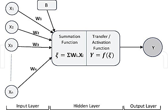
The activation function constitutes the second phase, wherein it takes the input signal from the summation function module and transforms it into the output of a node within an ANN model [14]. In general, each ANN comprises three fundamental components: node characteristics, network topology, and learning rules. Node characteristics govern signal processing by determining the number of associated inputs and outputs, the weights assigned to each input and output, and the activation function for each node. Learning rules dictate the initiation and adjustment of weights. Meanwhile, network topology defines the connectivity and organization of nodes. The operation of the ANN model involves computing the output of all neurons, representing a wholly deterministic calculation.
In this study, we will focus on two DL techniques: Long Short-Term Memory and Gate Recurrent Unit (GRU).
2.3. Long Short-Term Memory (LSTM)
LSTM stands for Long Short-Term Memory, and it functions as a network composed of interconnected neurons, each responsible for retaining previous state information [21]. With enough network elements, an LSTM network can conduct computations. The structure of an LSTM cell, depicted in Figure 6, comprises three key gates: the forget gate, the input gate, and the output gate. A distinctive aspect of LSTM networks is the memory cell, which serves as a repository for state information. Opening the input gate allows new information to be gathered into the cell, whereas opening the output gate leads to the erasure of past information. Within the feedback loop, the sigmoid function determines whether information should be preserved or deleted in the memory cell, while the hyperbolic tangent function manages the cell’s input and output. This amalgamation of functions empowers the LSTM to selectively retain or discard information, significantly enhancing its performance. This capability makes LSTMs particularly valuable for handling temporal datasets and making predictions [22]. Notably, in LSTM networks, the final cell is transmitted to the concluding stage solely when the output gate is opened. This specific behaviour unique to LSTMs prevents gradients from dissipating rapidly within the cell, resulting in improved performance in processing time series data and generating predictions compared to other approaches.

2.4. Gated Recurrent Unit (GRU)
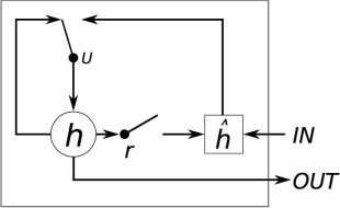
The GRU shares similarities with LSTM as it represents a more simplified and streamlined variant of the LSTM architecture. It was presented [23] by in 2014, at a time when the interest in recurrent networks was resurging within the relatively small research community. Just like the LSTM unit, the GRU possesses gating units that regulate information flow within the unit, yet it operates without distinct memory cells. The GRU lacks a mechanism to manage the extent of its state exposure, invariably revealing its entire state with each occurrence [24], [25]. Figure 7 represents the structure of the GRU model.
2.5. Forecasting Time
The prediction time is called the forecasting horizon [25]. Before designing the model, it is necessary to choose the appropriate forecasting horizon because the quality of the prediction is sensitive to the forecasting horizon. Prediction accuracy is influenced by the change in the forecast horizon, even with similar parameters in the same model. Figure 8 below explains the classification of PV power forecasting based on time.
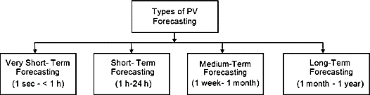
Very short-term (1sec – 1 h) forecasting is useful for real-time electricity transmission, optimal reserves, and power smoothing, while short-term (1h – 24 h) forecasting is useful for improving network security. By estimating the available electric power shortly, medium-term forecasting (1 week to 1 month) keeps the power system planning and maintenance schedule on track. Long- term forecasts (from one month to one year) aid in the planning of electricity generation, transmission, and distribution, as well as tendering and security operations.
2.6. Performance Evaluation of Forecasting Methods
Root Mean Square Error (RMSE), Mean Absolute Error (MAE), and the coefficient of determination (R2) are widely utilized performance metrics in PV power forecasting using machine learning approaches. RMSE quantifies the average error magnitude by taking the square root of the mean of squared differences between predicted values and observed outcomes [1]. On the other hand, MAE assesses the average significance of errors in a forecast dataset by averaging the differences between actual observations and predicted outcomes across the entire test sample, with each discrepancy assigned equal weight [1]. R2 provides a quantitative measure of the model’s predictive accuracy and its capability to offer reliable estimates of future PV power output. It is important to highlight that a predictive model demonstrates increased accuracy when both MAE and RMSE are minimized, and its efficiency is enhanced when R2 approaches a value of 1 [26]. The equations (2), (3) and (4) represent the expressions of RMSE, MAE and R2 respectively:
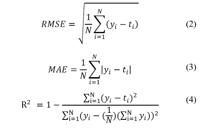
where yyii and ti are the measured and corresponding predicted values of PV power and N is the number of test samples.
2.7. Data Analysis
2.7.1. Problem Framing
The endeavour involves the application of deep learning techniques to develop grid-connected photovoltaic solar power facilities customized for the Sahelian climate. This segment focuses on accurately predicting solar PV power generation in Burkina Faso, as it plays a crucial role in effectively managing the intermittency of solar resources to enhance grid injection. Solar forecasting emerges as a highly cost-effective method for the seamless integration of solar energy. The process entails gathering historical data from a 2.3 MWp solar PV system at the Zagtouli PV Power plant and transforming it into a spreadsheet using Microsoft Excel. System coding will be implemented using Python, and data will be uploaded into the machine learning Toolbox for analysis.
2.7.2. Forecasting Input Variables
A set of variables were selected to perform the multivariate time series forecasting task. These variables are:
- Irradiance on an inclined plane (Irr);
- Global Horizontal Irradiance (GHI);
- Air temperature (Tair);
- Module temperature (Tm);
- PV Current (Ipv);
- PV Voltage (Vpv)
- Relative Humidity (RH);
- PV Power (Ppv)
- Title angle
- Wind direction (Wdire)
- Wind
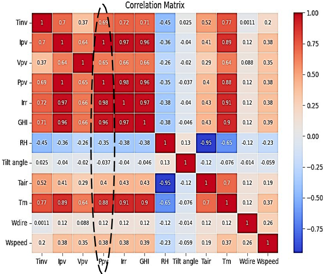
The Figure 9 clearly illustrates the correlation that exists between these various variables. The output variable is the output power of the PV system (Ppv), and we will focus on the correlation between this variable and others depicted in Figure 10. Thus, a strong correlation can be observed with the following variables: Ipv, Ppv, Irr, GHI, Tm, Tinv and Vpv. These variables will be used as inputs.
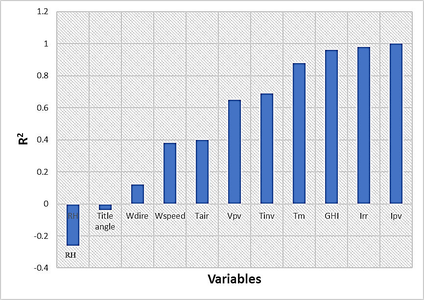
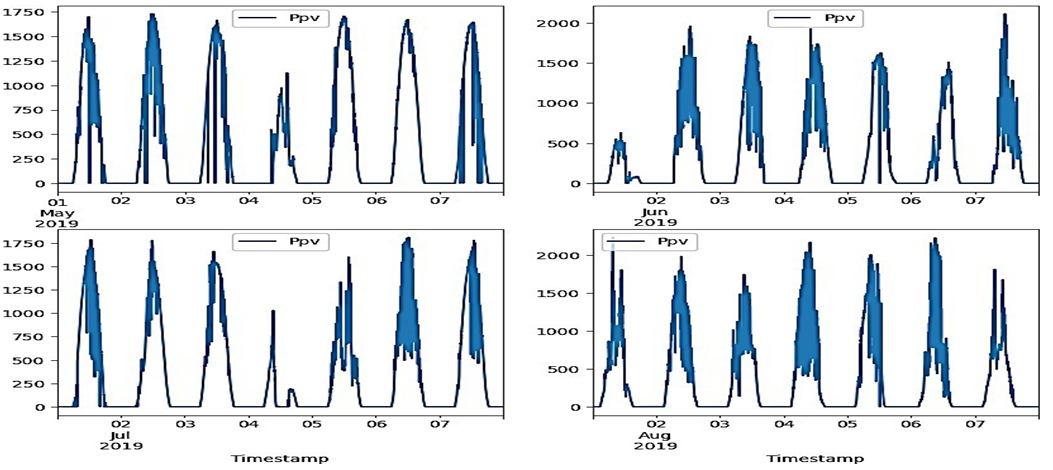
Figure 11 illustrates the daily PV power trend from the 2.3 MW solar PV system at the Zagtouli power plant in May, June, July, and August 2019. Some days, notably May 4th, July 1st, July 4th, and August 3rd, saw reduced output due to cloudy conditions.
2.7.3. Data Normalization
The data’s time series are all on distinct scales. To ensure that all of the features take small values on a similar scale, each feature was therefore independently normalized to have a mean of 0 and a standard deviation of 1. Because of their large range of values, target data were also normalized, just like input data. The following formula expressed by equation (5) was used to normalize the data:
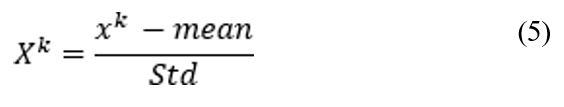
where Xk is the normalized value of series k, xxkk is the original input data value of series k, 𝑚𝑒𝑎𝑛 is the mean of the input data value of series k and 𝑆𝑡𝑑 is the standard deviation of the input data of series k.
3. Results and Discussions
3.1. Models Training and Testing
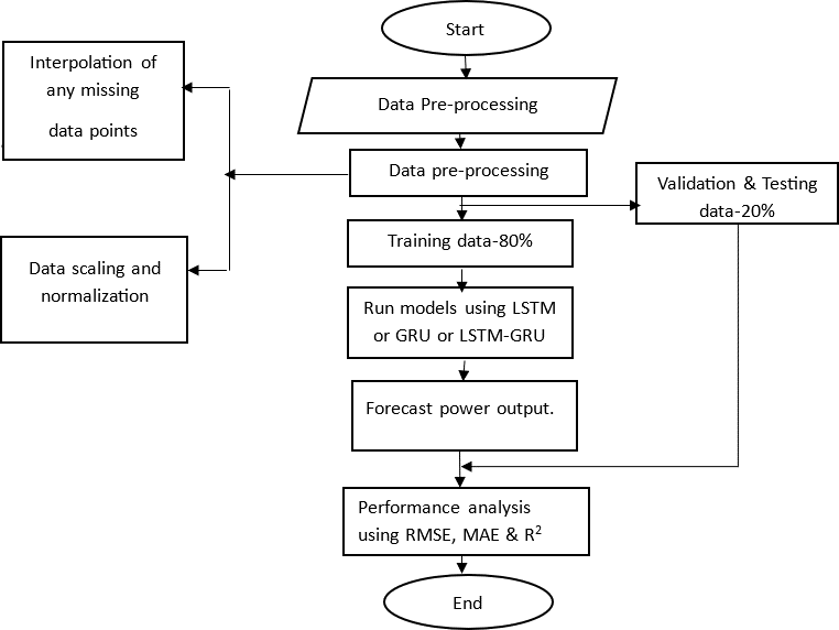
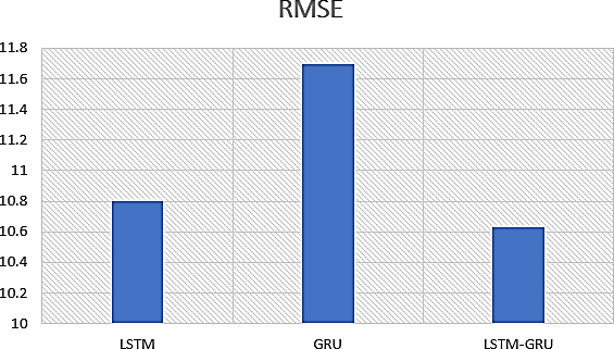
The Zagtouli Solar PV System’s power output was analysed using three distinct models. These models underwent training and evaluation using identical datasets for training, validation, and testing. Figures 13-15 depict the training and validation results of the LSTM, GRU, and LSTM-GRU models, respectively. The results demonstrate that the training loss curve is higher than the validation loss curve. That means the training data is more difficult to model than the validation data. The outcomes presented were achieved with the optimal hyperparameters detailed in Table 1. All models demonstrated commendable performance on the training and validation sets because lower training loss and validation loss indicate that the model fits the data correctly. Following the training phase, the finalized models were assessed using test sets, comprising data unfamiliar to the models. Unlike validation sets, test sets are utilized to gauge a trained model’s performance on previously unseen data. Table 2 provides a summary of the models’ test performances, measured with the RMSE, MAE and R2 metrics, after the training. Figure 16 clearly illustrates that the hybrid model (LSTM-GRU) outperforms, followed by the LSTM and GRU models, respectively.
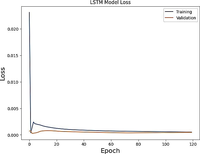
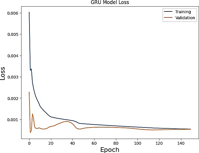
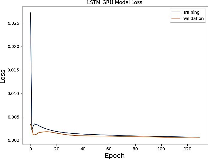
Table 1. Hyper-parameters
| Models | parameters | Epochs | Total Units |
| LSTM | 37531 | 120 | 91 |
| GRU | 34601 | 150 | 101 |
| LSTM-GRU | 85626 | 130 | 181 |
Table 2: Test Performances using LSTM, GRU and LSTM-GRU models
| Models | RMSE | MAE | R2 |
| LSTM | 10.799 | 2.09 | 0.998 |
| GRU | 11.695 | 2.1 | 0.997 |
| LSTM-GRU | 10.629 | 2.0 | 0.999 |
3.2. Solar PV Power Forecasting Using the Hybrid Model (LSTM-GRU)
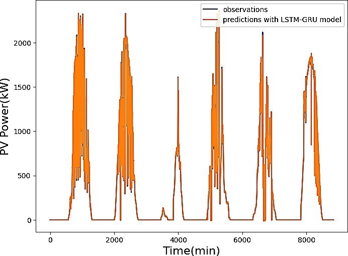
To implement the proposed models, a dataset comprising 176,940 records was gathered within the period of 00:00 to 23:59, with minute intervals, covering the period from May 1, 2019, to August 31, 2019. The training phase utilized 80% of the data, amounting to 141,552 data points, and spanned a total of 98 days. Validation involved 15% of the data, equivalent to 26,541 data points, spanning a potential 18-day period. Testing utilized 5% of the data corresponding to 8,847 data points, covering 6 days, specifically modelled for predictive analysis. These six days were employed to predict solar PV power, and the comparison between observed and predicted values was illustrated in Figure 17 using the LSTM-GRU model. Throughout this period, a noticeable overlap between the two curves indicates the model’s effectiveness in predicting the PV output power of Zagtouli’s solar power plant. Notably, deep learning models showcased superior performance compared to traditional models based on statistical series.
Table 3 below shows some of the results of predicting photovoltaic power output using hybrid deep learning models around the world. The results of predictions are very sensitive to the nature of the input data used, the hidden layers number as well as the duration and period during which data were collected [27]. Given the results of Table 3, we can conclude that the LSTM- GRU prediction model for Zagtouli’s solar power plant performs well.
Table 3. Comparison of some Hybrid deep learning models for PV Power Forecasting
| Year | Location | Horizon | Model | RMSE | Reference |
| 2019 | Alice Springs (Australia) | 1 day | LSTM- CNN | 13.82 | [28] |
| 2020 |
Nevada (USA) |
1 day |
LSTM- RNN |
6.29 | [8] |
| 2020 |
Limberg, (Belgium) |
45 min |
LSTM- CNN |
6.404 | [26] |
| 2021 | China | 1day |
VMD- ISSA- GRU |
1.5511 | [9] |
| 2021 | China | 1 day | GRUP | 6.83 | [29] |
| 2022 | Rabat (Morocco) | 1 day | LSTM- CNN | 6.65 | [30] |
| 2023 | Iran | 12 hours | GSA- LSTM | 10 | [31] |
| 2024 | Zagtouli (Burkina Faso) | 1 day | LSTM- GRU | 10.629 | Actual work |
4. Conclusion and Perspectives
Predicting solar PV power effectiveness presents a viable alternative for overseeing grid-connected PV solar plants. In this investigation, we employed two deep learning techniques and their combination to forecast a system at the Zagtouli PV plant site. The hybrid model (LSTM-GRU) demonstrated superior results compared to LSTM and GRU with the RMSE metric, recording values of 10.799, 11.695 and 10.629 respectively. The data utilized for this analysis were gathered from May 2019 to August 2019, corresponding to the rainy season. In the future, data from other seasons could be employed to compare performance outcomes. This research lays the groundwork for developing an efficient and intelligent digital platform for managing the inflow of injected solar PV power into Burkina Faso’s national electrical grid, aiming to secure the electrical network and optimize energy lost during continuous disconnections of power plants from the grid.
Conflict of Interest
The authors declare no conflict of interest.
Acknowledgements
The authors extend their gratitude to the University of Nairobi and Mohammed VI Polytechnic University for their valuable support, as well as to SONABEL for assisting in data collection at the Zagtouli PV Plant site. A special acknowledgement is also due to PASET RSIF for their financial contributions to this research endeavour.
- R. Ahmed, V. Sreeram, Y. Mishra, M.D. Arif, A review and evaluation of the state-of-the-art in PV solar power forecasting: Techniques and optimization, Renewable and Sustainable Energy Reviews, 124, 2020, doi:10.1016/j.rser.2020.109792.
- R.-E. Precup, T. Kamal, S.Z. Hassan, Solar Photovoltaic Power Plants, Springer Singapore, Singapore, 2019, doi:10.1007/978-981-13-6151-7.
- D.K. Dhaked, S. Dadhich, D. Birla, “Power output forecasting of solar photovoltaic plant using LSTM,” Green Energy and Intelligent Transportation, 2(5), 2023, doi:10.1016/j.geits.2023.100113.
- S. Sattenapalli, V.J. Manohar, “Research on Single-Phase Grid Connected PV Systems,” International Journal of Engineering and Advanced Technology, 9(2), 5549–5555, 2019, doi:10.35940/ijeat.b5159.129219.
- H. Sharadga, S. Hajimirza, R.S. Balog, “Time series forecasting of solar power generation for large-scale photovoltaic plants,” Renewable Energy, 150, 797–807, 2020, doi:10.1016/j.renene.2019.12.131.
- M. Elsaraiti, A. Merabet, “Solar Power Forecasting Using Deep Learning Techniques,” IEEE Access, 10, 31692–31698, 2022, doi:10.1109/ACCESS.2022.3160484.
- P. Li, K. Zhou, X. Lu, S. Yang, “A hybrid deep learning model for short-term PV power forecasting,” Applied Energy, 259(November), 114216, 2020, doi:10.1016/j.apenergy.2019.114216.
- F. Wang, Z. Xuan, Z. Zhen, K. Li, T. Wang, M. Shi, “A day-ahead PV power forecasting method based on LSTM-RNN model and time correlation modification under partial daily pattern prediction framework,” Energy Conversion and Management, 212, 2020, doi:10.1016/j.enconman.2020.112766.
- P. Jia, H. Zhang, X. Liu, X. Gong, “Short-Term Photovoltaic Power Forecasting Based on VMD and ISSA-GRU,” IEEE Access, 9, 105939–105950, 2021, doi:10.1109/ACCESS.2021.3099169.
- N.Q. Nguyen, L.D. Bui, B. Van Doan, E.R. Sanseverino, D. Di Cara, Q.D. Nguyen, “A new method for forecasting energy output of a large-scale solar power plant based on long short-term memory networks a case study in Vietnam,” Electric Power Systems Research, 199(June), 107427, 2021, doi:10.1016/j.epsr.2021.107427.
- A.P. Casares, “The brain of the future and the viability of democratic governance: The role of artificial intelligence, cognitive machines, and viable systems,” Futures, 103, 5–16, 2018, doi:10.1016/j.futures.2018.05.002.
- F. Chollet, Deep Learning with Python, 2nd Edition, Manning Publications Co, 2021.
- Dheeraj Mehrotra, Basics of Artificial Intelligence & Machine Learning, Notion Press, 2019.
- W. and A.H.Q. Salah Alaloul, Data Processing Using Artificial Neural Networks, Intechopen, 2020.
- R.C. Staudemeyer, E.R. Morris, “Understanding LSTM — a tutorial into Long Short-Term Memory Recurrent Neural Networks,” 2019.
- M. Hussain, M. Dhimish, S. Titarenko, P. Mather, “Artificial neural network based photovoltaic fault detection algorithm integrating two bi-directional input parameters,” Renewable Energy, 155, 1272–1292, 2020, doi:10.1016/j.renene.2020.04.023.
- R. Derakhshani, M. Zaresefat, V. Nikpeyman, A. GhasemiNejad, S. Shafieibafti, A. Rashidi, M. Nemati, A. Raoof, “Machine Learning-Based Assessment of Watershed Morphometry in Makran,” Land, 12(4), 2023, doi:10.3390/land12040776.
- A. Shah, M. Shah, A. Pandya, R. Sushra, R. Sushra, M. Mehta, K. Patel, K. Patel, A comprehensive study on skin cancer detection using artificial neural network (ANN) and convolutional neural network (CNN), Clinical EHealth, 6, 76–84, 2023, doi:10.1016/j.ceh.2023.08.002.
- N. V. Ranade, V. V. Ranade, “ANN based surrogate model for key Physico-chemical effects of cavitation,” Ultrasonics Sonochemistry, 94, 2023, doi:10.1016/j.ultsonch.2023.106327.
- R. Langbauer, G. Nunner, T. Zmek, J. Klarner, R. Prieler, C. Hochenauer, “Modelling of thermal shrinkage of seamless steel pipes using artificial neural networks (ANN) focussing on the influence of the ANN architecture,” Results in Engineering, 17, 2023, doi:10.1016/j.rineng.2023.100999.
- C.H. Liu, J.C. Gu, M.T. Yang, “A Simplified LSTM Neural Networks for One Day-Ahead Solar Power Forecasting,” IEEE Access, 9, 17174–17195, 2021, doi:10.1109/ACCESS.2021.3053638.
- N.L.M. Jailani, J.K. Dhanasegaran, G. Alkawsi, A.A. Alkahtani, C.C. Phing, Y. Baashar, L.F. Capretz, A.Q. Al-Shetwi, S.K. Tiong, Investigating the Power of LSTM-Based Models in Solar Energy Forecasting, Processes, 11(5), 2023, doi:10.3390/pr11051382.
- K. Cho, B. van Merrienboer, D. Bahdanau, Y. Bengio, “On the Properties of Neural Machine Translation: Encoder-Decoder Approaches,” 2014.
- J. Chung, C. Gulcehre, K. Cho, Y. Bengio, “Empirical Evaluation of Gated Recurrent Neural Networks on Sequence Modeling,” 2014.
- M.N. Akhter, S. Mekhilef, H. Mokhlis, N.M. Shah, “Review on forecasting of photovoltaic power generation based on machine learning and metaheuristic techniques,” IET Renewable Power Generation, 13(7), 1009–1023, 2019, doi:10.1049/iet-rpg.2018.5649.
- G. Li, S. Xie, B. Wang, J. Xin, Y. Li, S. Du, “Photovoltaic Power Forecasting with a Hybrid Deep Learning Approach,” IEEE Access, 8, 175871–175880, 2020, doi:10.1109/ACCESS.2020.3025860.
- S. Theocharides, G. Makrides, A. Livera, M. Theristis, P. Kaimakis, G.E. Georghiou, “Day-ahead photovoltaic power production forecasting methodology based on machine learning and statistical post-processing,” Applied Energy, 268, 2020, doi:10.1016/j.apenergy.2020.115023.
- K. Wang, X. Qi, H. Liu, “A comparison of day-ahead photovoltaic power forecasting models based on deep learning neural network,” Applied Energy, 251, 2019, doi:10.1016/j.apenergy.2019.113315.
- Y. Qu, J. Xu, Y. Sun, D. Liu, “A temporal distributed hybrid deep learning model for day-ahead distributed PV power forecasting,” Applied Energy, 304, 2021, doi:10.1016/j.apenergy.2021.117704.
- A. Agga, A. Abbou, M. Labbadi, Y. El Houm, I.H. Ou Ali, “CNN-LSTM: An efficient hybrid deep learning architecture for predicting short-term photovoltaic power production,” Electric Power Systems Research, 208, 2022, doi:10.1016/j.epsr.2022.107908.
- D. Sadeghi, A. Golshanfard, S. Eslami, K. Rahbar, R. Kari, “Improving PV power plant forecast accuracy: A hybrid deep learning approach compared across short, medium, and long-term horizons,” Renewable Energy Focus , 45, 242–258, 2023, doi:10.1016/j.ref.2023.04.010.
No. of Downloads Per Month