1. Introduction

This paper is an extension of work originally presented at the 3rd International Symposium on Electrical, Electronics, and Information Engineering (ISEEIE 2023) [1].

A long-standing problem in Japanese agriculture is the aging and decline of farmers. According to a survey, from 2015 to 2020, the number of farmers decreased by approximately 22% to 1,363,000, and the percentage of those aged 65 years or older increased by 5% to 69.6% [2]. The main causes of this are that appropriate farm work requires tacit knowledge and much human labor. Regarding the former, appropriate work is based on the heuristics of experts; therefore, it is difficult to share. Regarding the latter, Japan’s agricultural fields are small, and mechanization has not yet progressed. These problems create barriers for new farmers and lead older farmers to quit farming. To solve this problem, “Smart Agriculture” is being promoted. Specifically, production management systems and the automatic operation of agricultural machinery are expected to clarify and save labor in farm work. However, these technologies are expensive and difficult to implement by farmers. Therefore, in this study, crop monitoring using unmanned aerial vehicles (UAV) was adopted, which is more reasonable than other technologies.

In UAV monitoring, multispectral cameras are often used to obtain the sunlight reflectance of crop leaves in various bands. Generally, healthy crops have high reflectance in the near-infrared band and low reflectance in the red band. However, in stressed crops, the difference in reflectance between the two bands decreases, as shown in Figure 1 [3], [4]. Based on this reflection characteristic, many vegetation indices (VI) have been developed using calculation formulas to understand vegetation conditions [5]. For example, using VIs, studies have created rice yield maps using the Normalized Difference Vegetation Index (NDVI) and the Normalized Difference Red Edge Index (NDRE) [6], [7]. These studies have shown that the VI value in the young panicle formation stage and the heading stage are correlated with yield; therefore, yield prediction is possible. However, these predictive models cannot be applied everywhere but within the research environment. Furthermore, despite multiple monitoring sessions, the model predicted using only the VI value input during the heading stage. In Japan, yield is important for planning rice demand and supply. Therefore, early and highly accurate predictions with numerous features are required.

This study focused on additional fertilization during farming. This study is important because it directly influences growth and yield. Generally, this work is conducted between the young panicle-forming and heading stages to supply nitrogen and potassium and can be expected to increase yield by enriching the contents of ears [8]. However, excessive fertilizer causes lodging owing to overgrowth, releasing water from the roots due to osmotic pressure, and health hazards owing to nitrate-nitrogen dissolution into groundwater [9], [10]. For nitrate-nitrogen, the Japanese standard value for water pollution is set at 10 mg/L [11]. Based on these negative effects, it is necessary to determine the appropriate amount of fertilizer and apply variable fertilization. Because the effect of farm work appears gradually, it is important to compare it before and after work. Therefore, in this study, we use a new method of time-series analysis of VIs obtained from a UAV to visualize the vegetation before and after additional fertilization and analyze the appropriate fertilization amount. Furthermore, to reduce the workload of UAV monitoring, we use random forest (RF) to minimize the monitoring period.

2. Method

2.1. Monitoring

The monitoring targeted paddy fields owned by private farmers in Hanamaki City in Iwate Prefecture, Japan, and yielded 10 analysis results for six sites from 2021 to 2023 [1], [12], [13]. Several sites were used in the experiment, and the additional fertilizer amount varied for each field. This is because growth differences were observed for each fertilizer amount.

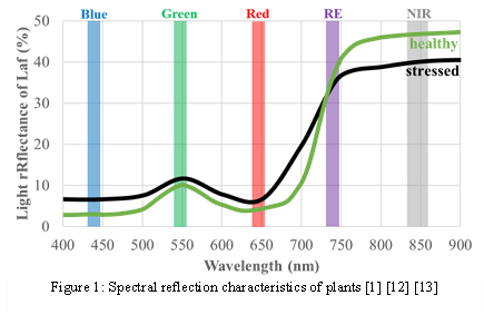
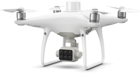
Table 1 shows the sites and cropping information where the comparative fertilizer application experiments were conducted (Yuguchi-8 in 2022 and Yuguchi in 2023). The distance between the two fields was approximately 1 km; therefore, the weather conditions were similar. Both fields are adjacent to each other and can be divided into North, Center, and South in Yuguchi-8, and West, Center, and East in Yuguchi. Fertilizer amounting to 2.8, 3.5, and 4.2 gN/m² was applied in the middle of July using a pesticide spraying UAV (AGRAS MG-1, DJI Co., Ltd. [14]).

To calculate the VI, a UAV equipped with a multispectral camera is required. Thus, a UAV (Phantom 4 Multispectral, DJI Co., Ltd.), shown in Figure 2 was used. It weighs 1,487 g, has a maximum flight time of 27 min, and has a multispectral camera with one RGB sensor for visible light and five monochrome sensors for multispectral light. The bands of the monochrome sensor were 450 nm (blue), 560 nm (green), 650 nm (red), 730 nm (red edge: RE), and 840 nm (near-infrared: NIR) [15]. The flight altitude was set to 30 m, and orthogonal images of each band were created after monitoring. The VI values were then calculated from these orthoimages. The VIs calculated in this study were (1), (2), and (3).

The NDVI was used for vegetation diagnosis. This was calculated by normalizing the NIR and Red bands. It is widely used; however, it has been reported that the soil easily affects it, and the index becomes saturated during the peak vegetation season [6], [16], [17]. The NDRE was used to diagnose crop stress and nitrogen content. The RE band reaches deeper into the canopy than the Red band; therefore, stress can be detected earlier. Additionally, it is not easily saturated; therefore, depending on the season, it may be more appropriate than NDVI for diagnosing vegetation and yield [7], [17], [18]. A Standardized Normalized Difference Red Edge Index (sNDRE) was developed to ensure that the NDRE did not change unless it was under significant stress. This is the relative value for each date and is used for a relative comparison within a field [1], [12], [13]. In addition, it uses only NDRE for calculations, and it is possible to diagnose the relative stress and nitrogen content levels in the field.

After computing these three VIs, meshes were created in the rice field portion of the orthoimage. The mesh size was 3 m square.

The VI of each mesh was determined as the average VI value of pixels within the mesh. After computing the VIs of all meshes on all monitoring dates, VI time-series data were generated for each mesh.

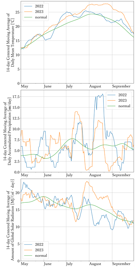
Figure 3 shows the 14-day centered moving average of the daily mean temperature, accumulated precipitation, and global solar radiation at Yuguchi during the rice-growing period (May to September) in 2022, 2023, and a normal year. As a characteristic point, there was heavy rainfall in August 2022 and high temperatures in 2023. To adjust for these weather differences, monitoring dates were converted to growth stages using the Effective Accumulated Temperature (EAT) from the transplantation date and paddy rice growth model [19], [20]. Table 2 shows the correspondence between the EAT and growth stages, and Figure 4 shows the relationship between the growth stages and dates for both years.

2.2. Evaluation of Additional Fertilization

To visualize the fertilization effect, this research used time- series clustering (TSC) with the K-Means++ method on the VI time-series data presented in Section 2.1. Clustering usually classifies 2 or 3-dimensional data which can be shown in scatter diagrams [21]. However, this analysis aimed to classify time-series data. Therefore, a program was developed to handle time-series data with several missing monitoring dates [1]. This program is an improved version of the function “TimeSeriesKMeans” [22] in the Python library “tslearn.” This program was used in this research to conduct TSC. The elbow method [1], [23] was used to determine the number of clusters. From the TSC results, the VI time-series transition of each cluster’s centroid, cluster distribution, and cluster ratio for each paddy field were obtained. Based on these results, we determined the growth differences according to the fertilizer amount and the appropriate fertilizer amount. Furthermore, a crop estimate by unit acreage sampling was conducted immediately before harvest to confirm the consistency between the appropriate fertilizer amount determined by TSC analysis and the actual yield. The sampling method was to select five meshes per field so that the heading-stage NDVI was scattered, and five stubbles per mesh were collected. The selected meshes are listed in Table 3.

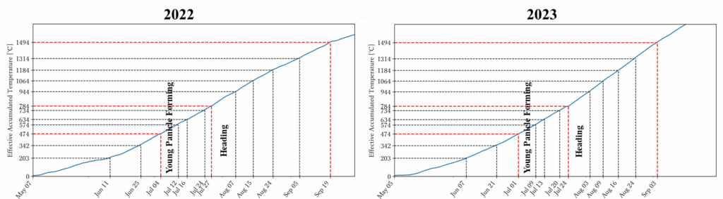
Table 2: Correspondence between growth stage and EAT

2.3. Optimization of Monitoring Period

Previous studies have analyzed healthy vegetation growth, stress, etc. in paddy rice using the TSC of VI time-series data [12], [13]. However, UAV monitoring, such as moving to sites, preparing for flight, and computing VI values from aerial photographs, takes time. Therefore, a survey was conducted to identify the subset of monitoring dates for which the feature quantity was not reduced significantly [1]. RF was used in this survey. This was adopted because it can handle the categorical values that are the output results of TSC (i.e., cluster ID) and it outputs the importance of each independent variable (monitoring date).The execution conditions for RF are listed in Table 4 [1]. From the RF, a classifier model was created that outputs the cluster ID when given the VI time-series data of each mesh. The optimization method is shown in Figure 5. First, a classifier was created using the training data of the VI time series over the entire period (Entire RF). Second, the optimized period was determined based on the importance of the test data given to the classifier. Third, another classifier was created using the training data of the VI time series values in the optimized period (Optimized RF). Fourth, the cluster ID match percentages were calculated when classifying the test data between the TSC and Entire RF (𝑝𝑝𝑝𝑝𝑅𝑅𝑅eee) and between the TSC and Optimized RF ( 𝑝𝑝𝑝𝑝_{𝑜𝑜𝑜𝑜ee}). Finally, the McNemar’s test was performed with the null hypothesis as “𝑝𝑝_{𝑅𝑅𝑅eeee} =ppoooee’’ and it was evaluated that optimization was successful if the null hypothesis was not rejected. Using this method, the optimized period was determined from the monitoring data of eight sites (excluding the two sites in Table 1 from the monitoring data of all ten sites). This confirmed the consistency between the appropriate fertilizer amount using TSC analysis results in the optimized period and the actual yield.

3. Results

3.1. Comparison of Additional Fertilizer Amounts

Table 5 presents the yields of the five sampled meshes at both sites. Sample 5 from West of Yuguchi was missing because the survey was discontinued. The sampled yield was calculated as the weight of five stubbles. These units were converted to SI units, and the average for each rice field is shown in the second line from the bottom. The bottom line shows the p-value of the Kruskal-Wallis test (non-parametric, unpaired, differences between three or more groups) with the null hypothesis set as “the average of sampled yields of all rice fields are equal.” As a result, the null hypothesis was adopted even at the 10% significance level, as the p-value for both sites significantly exceeded 0.1.

For the entire TSC period, the time-series transitions in each cluster centroid, cluster ID distribution map, and percentage of each cluster are shown in Table 6, Table 7, and Table 8. For Yuguchi-8 in 2022, the meshes were classified into two, three, and three clusters for NDVI, NDRE, and sNDRE, respectively. For the NDVI, there was no difference between clusters in the heading stage, and the yields were expected to be similar in all rice fields. In the NDRE, differences were observed at the heading stage, but no differences were observed thereafter. Cluster-0, which had relatively low stress, was found near the ridges. In sNDRE, Cluster-0 was high and often observed near the ridge. The central meshes of each paddy field were many Clusters-1 and Cluster-2, but after heading, the value did not differ by more than 0.5, with no difference in the stress level. The same can be said for all three rice fields, and no growth differences were observed between them. Therefore, the appropriate fertilizer amount was analyzed as the north field (2.8 gN/m²), where the amount is the lowest, considering fertilizer costs etc.

Table 3: Sampled meshes

Table 4: Execution conditions of RF

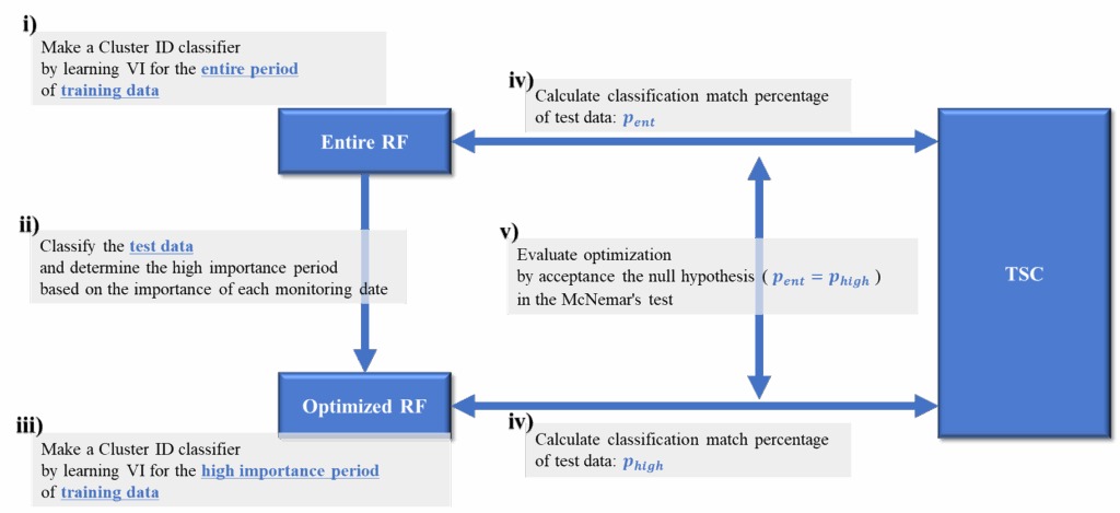
Table 5: Yields of 5 sampled meshes and results of Kruskal-Wallis test

At Yuguchi in 2023, the meshes were classified into three, three, and four clusters for NDVI, NDRE, and sNDRE, respectively. In the NDVI, there was a difference of approximately 0.15 between clusters at the first monitoring. However, the low value (Cluster-2) improved because of the fertilizer. Thus, it was concluded that there was no difference in growth between the fields because the value of each cluster was similar at the heading stage. There was a large difference in sNDRE between the four clusters. Similar to other VI, high-value (Cluster-0 and Cluster-1) were observed at the center of the field. These two clusters appeared slightly more frequently in the West and Center. Similar to Yuguchi-8, the same was observed for all three fields, but no growth differences were observed. Therefore, the appropriate amount of fertilizer was analyzed in the western field (2.8 gN/m²).

Table 6: Centroid of each cluster (entire period)

3.2. Optimization of Monitoring Period

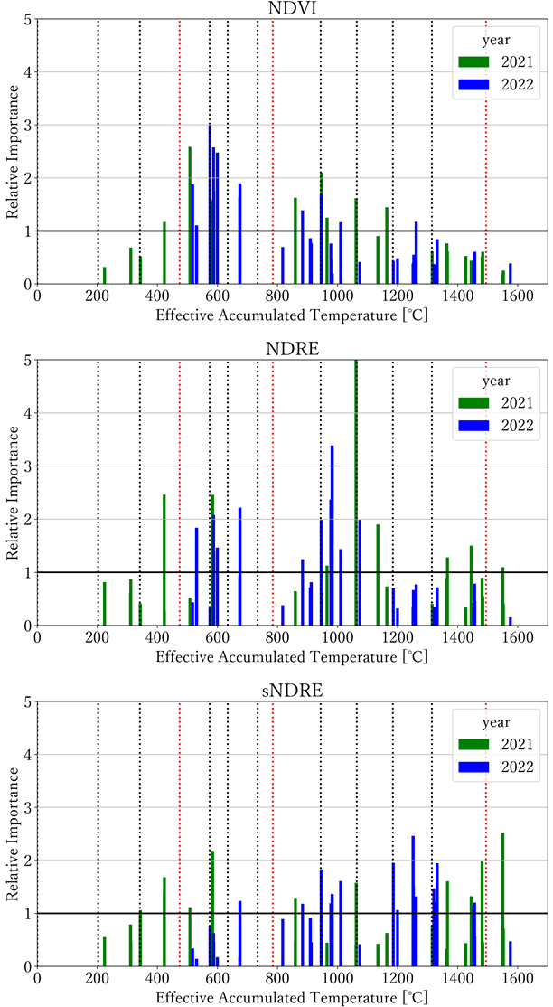
The importance results for the six sites (excluding Yuguchi-8 in 2022 and all sites in 2023) are shown in Figure 6. The vertical axis in this figure represents the Relative Importance. The Importance output by the RF is the percentage contribution [1], [24]. That is, the fewer the monitoring dates, the higher the value. To adjust for this, Relative Importance was calculated by dividing the usual output importance by the reciprocal of the number of monitoring dates [1] [24]. To optimize the optimization method of monitoring period, first, the initial period was extracted, for which the minimum period included all data with a Relative Importance of one or more. Next, the period was expanded or deduced to the sum of the Relative Importance of 49% to 51%, in contrast to the entire period shown in Figure 6.

Table 7: Cluster ID distribution map (entire period)

Table 8: Percentage of each cluster (entire period)

The optimized periods of the EAT determined using this method are listed in Table 9. The rightmost column shows the EATs of the optimized period converted to dates using the EAT from May 7 in a normal year. The optimal period for all VIs was approximately one month. This period was from the young panicle forming to the milk ripe for NDVI and NDRE, and from heading to the full ripe for sNDRE.  In Table 10, the results are applied to two sites that were excluded when calculating the optimized period (i.e., Yuguchi -8 in 2023 and Yuguchi in 2022). For the match rate of the cluster ID classification of the test data between the Entire RF and TSC (), and the Optimized RF and TSC (),  was greater than . They are not necessarily 100% because the training data comprise 25% of all the meshes and the remaining 75% of the test data. The rightmost column shows the p-value of the test for the difference between two percentages. No VI was significant at the 5% level. In other words, the monitoring period can be optimized without significantly reducing the classification accuracy. In addition, although the 2023 data were not used to derive the optimized period,  of Yuguchi had high accuracy (over 98%). This indicates that the optimized period can be derived using the EAT without depending on the year.

4. Discussion

4.1. Visualization of Paddy Rice Growth

In the TSC during the optimized period, most results showed that growth was different in the center of the fields and near the ridge. In the NDVI and NDRE, the area near the ridge was classified into low-value clusters, so it is thought that the vegetation growth and stress states were not better than those in the center of the field. In contrast, for the sNDRE at Yuguchi-8, the near-ridge meshes were classified into high-value clusters. It is thought that the amount of nitrogen was high because the fertilizer was washed away by heavy rain in August, (Figure 3, Table 7).

However, at Yuguchi-8, all monitoring occurred after heading, and at Yuguchi, the first time was before young panicle formation and the second time during heading. In short, no monitoring was conducted between the start date of the optimized period and the fertilization date at either site. From the results of the optimized TSC period, it was not possible to visualize the growth before fertilization. Thus, vegetation differences are discussed using the results for the entire period (Table 6). From the time-series trends of each cluster, it can be seen that NDVI and NDRE increased between the first and second monitoring days. This suggests that nutrient supplementation with fertilizers improves vegetation and stress conditions. In addition, sNDRE is not suitable for comparing these conditions with other days because of the standardization of each day.

Table 9: Optimized period of EAT of each VI

As described above, TSC of the VIs was able to visualize the health status of paddy rice and predict the appropriate fertilizer amount. On the other hand, in order to further improve predictive.

Table 10: Results of mesh classification match percentage between RF and TSC and McNemar’s test

For vegetation growth changes before and after fertilization, there were no monitoring data before fertilization included in the optimized period for either field (Table 6, Table 9).

Usually, additional fertilization is conducted on a day when EAT is around 500 to 650 (about 2 to 4 weeks before heading). Although sNDRE was not included in this period, NDVI and power, the following two things need to be considered. The first is the use of a broader range of wavelengths beyond visible light. Some of the VIs that have been developed so far use these bands (e.g., NDNI, CAI, etc.) [5], [25]. By using these VIs after confirming their effectiveness with ground truth data such as RGB images and site inspections, it becomes possible to visualize water stress, nutritional deficiencies, pest infestation, and so on. For ensuring the accuracy and reliability, it is necessary to verify them using detailed measurement data obtained from sensors such as air temperature and water temperature in mesh unit. Future research should utilize such ground truth data for TSC to observe various aspects of crop conditions. The second is to perform accurate spatial analysis. In this paper, for fast processing, the data used in the TSC was reduced in size by determining the mesh size (approximately 3m x 3m) based on the resolution. It is desirable to perform TSC with various mesh sizes and verify the mesh size that increases the accuracy of the optimal fertilizer amount prediction and yield prediction. Also, the spatial variability of vegetation indices within the rice field and its implications for fertilizer management may be caused by the evenness of the rice field, location of water outlets and water flow within the rice field, and so forth. We hope to identify the causes of this spatial heterogeneity using spatial analysis techniques and the analytical methods of this study.

4.2. Evaluation of Optimization

In the previous section 4.1, it was analyzed in both fields that the appropriate fertilizer amount was the lowest amount field by the TSC using the optimized period. The bottom panel of Table 5 shows the evaluation of this analysis from the viewpoint of yield. As mentioned in the previous chapter, this is the p-value of the test for significant differences in yield between fields when the null hypothesis is set as “the average of sampled yields of all rice fields are equal.” Based on this test, the null hypothesis was adopted, even at the 10% significance level. In other words, it cannot be said that there is a difference in yield between paddy fields, and it also cannot be said that changing the fertilizer amount will change the yield. Therefore, the field with the least amount of fertilizer is appropriate from the viewpoint of avoiding fertilizer costs, excessive fertilization, and environmental impacts. This result agrees with the TSC analysis results.

In local practice, the fertilizer applied to all fields is 4.2 gN/m². Assuming that this was changed to an appropriate 2.8 gN/m², the fertilizer was reduced to 87 and 91 kg, and the amount of leached nitrogen was reduced to 0.070mg/L for both Yuguchi-8 and Yuguchi. It was small compared to the water pollution standards. This is the case when fertilizer is applied during irrigation, and the leaching amount is only approximately 3% of that during surface drainage [26], [27][28]. Therefore, TSC method reduces the amount of excess fertilizer used, so it is expected to reduce the environmental impact. Furthermore, the development of such appropriate fertilization techniques will contribute to the sustainability of agriculture by creating soil that can produce food over the long-term without degrading the environment [29]. And continued analysis of this study will promote long-term soil health by reducing chemical fertilizers and increasing organic ones without reducing yields. This is a topic for future work.

As described above, the amount of excess fertilizer was estimated by using TSC for VI from UAV. In order to ensure accuracy and reliability, this research will need to address the following three things in the future. First is the use of data fusion technology. This is important to enhance the predictive power of the model and provide a more comprehensive understanding of factors influencing crop response to fertilization. Future research would like to try to analyze differences in soil and past crop management practices for each rice field.

5. Conclusions

In this research, the VIs time-series data were obtained using a UAV. Additionally, the monitoring dates were converted into growth stages (EAT) using a paddy rice growth model from related research [19], [20]. On this data, three analyzes were performed. In the first analysis, it was possible to visualize healthy vegetation growth and stress in paddy rice using the TSC. We also confirmed that healthy vegetation growth and stress of crops were improved by fertilizer. In the second analysis, the Kruskal–Wallis test confirmed the appropriate amount from the results of TSC. In the third analysis, the optimized period was determined based on the importance of each independent variable using RF. Based on these findings, our work have discovered the technologies can help reduce fertilizer costs, excessive fertilization and environmental impacts, and promote the use of UAV.

A future challenge is the development of a growth-prediction model. This study deals with ex-post evaluations, such as the visualization and classification of crop conditions. Also iIt is necessary to make future predictions for crop yields, early disease detection, and variable fertilization using VIs. Currently, there are no absolute standards for VIs, and no study has been found that generalizes the desirable values at each growth stage. However, a research has established a target NDVI for each growth stage using a portable device for NDVI measurement [30], [31]. This study collects and analyzes VI data via UAVs to improve productivity and reduce costs. For this purpose, we will develop a system that uses deep learning to provide decision support for fertilization in natural language based on the features of monitoring images [32] and methods such as farm income prediction based on yield prediction using regression, and so on. Then, it would be desirable to be able to connect UAVs with these systems and provide information to farmers in real time. As the IoT advances, security issues are a concern, so it will be important to develop autonomous decentralized systems that increase data tamper resistance using blockchain technology [33], [34], [35], [36].

Conflict of Interest

The authors declare no conflict of interest.

Acknowledgment

The authors would like to thank the Research Center for Industrial Science and Technology, Iwate University, and the farmers in the experimental field for providing monitoring and yield survey data. We would also like to thank Editage (www.editage.jp) for English language editing. Finally, we are grateful to the referees for their helpful comments.

1. T. Ito, K. Minamino and S. Umeki, “Analysis of Vegetation Indices by Time Series Clustering of Drone Rice Monitoring Data,” 3rd International Symposium on Electrical, Electronics and Information Engineering (ISEEIE 2023), 2023, DOI: 10.1049/icp.2023.1853
2. Ministry of Agriculture, Forestry and Fisheries, “2020 nen nou-rin-gyou census kekka no gaiyou (kakuteichi),” URL: https://www.maff.go.jp/j/tokei/kekka_gaiyou/noucen/2020/index.html, [Accessed 5 February 2024], (article in Japanese).
3. K. Miyama, “Nou-sakumotsu · dozyou no bunkou-hansya-tokusei – nou- you-chi he no remote sensing gizyutsu no tekiyou-sei (I),” Journal of the Agricultural Engineering Society, Japan, 56(12):1197-1202, 1988, (article in Japanese).
4. J. L. Hatfield and J. H. Prueger, “Value of Using Different Vegetative Indices to Quantify Agricultural Crop Characteristics at Different Growth Stages under Varying Management Practices,” Remote Sensing, 2(2):562-578, 2010, DOI: 10.3390/rs2020562.
5. J. Xue and B. Su, “Significant Remote Sensing Vegetation Indices: A Review of Developments and Applications,” Journal of Sensors, 2017:1-17, 2017, DOI: 10.1155/2017/1353691 T. Ito et al. / Advances in Science, Technology and Engineering Systems Journal Vol. 9, No. 3, 29-40 (2024) www.astesj.com 40
6. K. Tanaka and A. Kondoh, “Mapping of Rice Growth Using Low Altitude Remote Sensing by Multicopter,” Journal of The Remote Sensing Society of Japan, 36(4):373-387, 2016, DOI: 10.11440/rssj.39.S1.
7. K. Harashina, K. Yamamoto, M. Maki, Y. Muto and E. Kurashima, “Monitoring Growth of Water-seeded Rice in Tsunami-stricken Paddy Fields Using UAV-mounted Multispectral Sensor,” Journal of the Japanese Society of Irrigation, Drainage and Rural Engineering, 87(2):121-126, 2019, (article in Japanese with a title in English).
8. A. Matsuzaki, Inasaku dai hyakka dai 2 han dai 3 kan saibai no zissai/sehi- gizyutsu, Rural Culture Association, 2004, (article in Japanese).
9. Kubota Co., Ltd., “Mizu to hiryou ni yoru control | tanbo no kanri to higai- taisaku | okome ga dekirumade | Kubota no tanbo [manannde tanoshii! tanbo no sougou zyouhou site],” URL: https://www.kubota.co.jp/kubotatanbo/rice/management/manure.html, [Accessed 21 December 2023], (article in Japanese).
10. National Institute of Science and Technology Policy, “NISTEP PDF cover 200612,” URL: https://nistep.repo.nii.ac.jp/record/5536/files/NISTEP- STT069.pdf, [Accessed 21 December 2023], (article in Japanese).
11. Ministry of the Environment, “Suishitsu-osen ni kakawaru kankyo-kizyun,” URL: https://www.env.go.jp/kijun/mizu.html, [Accessed 7 February 2024], (article in Japanese).
12. T. Ito, K. Minamino and S. Umeki, “Analysis of Vegetation Indexes by Time Series Clustering of Drone Rice Monitoring Data,” The 21st Forum on Information Technology (FIT2022), 21(4):105-110, 2022, (article in Japanese with a title in English).
13. T. Ito, K. Minamino and S. Umeki, “Analysis of Fertilization Effects on Rice and Wheat by Time-Series Clustering of Vegetation Index Data,” Proceedings of the 5th International Symposium on Advanced Technologies and Applications in the Internet of Things (ATAIT 2023), 2023.
14. Da-Jiang Innovations Science and Technology Co., Ltd., “AGRAS MG-1S Series – DJI,” URL: https://www.dji.com/mg-1s, [Accessed 8 February 2024].
15. Da-Jiang Innovations Science and Technology Co., Ltd., “P4 MultispectralDJI,” URL: https://www.dji.com/p4-multispectral, [Accessed 8 February 2024].
16. A. Karnieli, N. Agam, R. T. Pinker, M. Anderson, M. L. Imhoff, G. G. Gutman, N. Panov and A. Goldberg, “Use of NDVI and Land Surface Temperature for Drought Assessment: Merits and Limitations,” Journal of Climate, 23(3):618-633, 2010, DOI: 10.1175/2009JCLI2900.1
17. H. Zheng, W. Ji, W. Wang, J. Lu, D. Li, C. Guo, X. Yao, Y. Tian, W. Cao,
    Y. Zhu and T. Cheng, “Transferability of Models for Predicting Rice Grain Yield from Unmanned Aerial Vehicle (UAV) Multispectral Imagery across Years, Cultivars and Sensors,” Drones, 6(12:423):1-19, 2022, DOI: 10.3390/drones6120423.
18. L. Osborn, “NDVI vs. NDRE: What’s the Difference? – Sentera,” URL: https://sentera.com/resources/articles/ndvi-vs-ndre-whats-the-difference/, [Accessed 8 February 2024].
19. E. Kanda, Y. Torigoe and T. Kobayashi, “A Model to Estimate the Increase of Leaf Number on the Main Culm of the Rice Plant,” Japanese Journal of Crop Science, 69(4):540-546, 2000, DOI: 10.1626/jcs.69.540, (article in Japanese with an abstract in English).
20. E. Kanda, Y. Torigoe and T. Kobayashi, “A Simple Model to Predict the Developmental Stages of Rice Panicles Using the Effective Accumulative Temperature,” Japanese Journal of Crop Science, 71(3):394-402, 2002, DOI: 10.1626/jcs.71.394, (article in Japanese with an abstract in English).
21. A. K. Jain, M. N. Murty and P. J. Flynn, “Data Clustering: A Review,” ACM Computing Surveys, 31(3):264-323, 1999, DOI:10.1145/331499.331504.
22. R. Tavenard, “tslearn.clustering.TimeSeriesKMeans — tslearn 0.6.3 documentation,”URL:https://tslearn.readthedocs.io/en/stable/gen_modules/clus tering/tslearn.clu stering.TimeSeriesKMeans.html
23. C. Shi, B. Wei, S. Wei, W. Wang, H. Liu and J. Liu, “A quantitative discriminant method of elbow point for the optimal number of clusters in clustering algorithm,” EURASIP Journal on Wireless Communications and Networking, 31:1-16, 2021, DOI: 10.1186/s13638-021-01910-w.
24. S. Ronaghan, “The Mathematics of Decision Trees, Random Forest and Feature Importance in Scikit-learn and Spark,” URL: https://towardsdatascience.com/the-mathematics-of-decision-trees- random- forest-and-feature-importance-in-scikit-learn-and-spark-f2861df67e3, [Accessed 11 February 2024].
25. The IDB Project, “Index DataBase,” URL: https://www.indexdatabase.de/, [Accessed 23 April 2024].
26. Toyama Prefecture, “Chika-sui kanyou no suishin ni mukete ,” URL: https://www.pref.toyama.jp/documents/7739/00745883.pdf, [Accessed 17 February 2024], (article in Japanese).
27. C. Imagawa, “Nitrogen Dynamics Modeling to Support Land and Water Management in Rice Paddy Watershed,” Soil/Water Research Group Materials, 30, 2013, (article in Japanese with a title in English).
28. M. Tsuji and M. Takei, “Degrees of Water Purification in Cultivated Rice Fields and Fallow Fields,” Research bulletin of the Aichi-ken Agricultural Research Center, 43:1-6, 2011, (article in Japanese with an abstract in English).
29. M. M. Tahat, K. M. Alananbeh, Y. A. Othman and D. I. Leskovar, “Soil Health and Sustainable Agriculture,” Sustainability, 12(12), 2020, DOI: 10.3390/su12124859.
30. NIKON-TRIMBLE CO., LTD.,”GreenSeeker 2,” URL:https://www.nikon-trimble.co.jp/products/product_detail.html?tid=428, [Accessed 15 February 2024].
31. Y. Kaneta, M. Nishida, F. Takakai and T. Sato, “New growth diagnosis standards of high-yielding rice and demonstration of high yielding using NDVI by GreenSeeker handheld crop sensor,” Japanese Journal of Soil Science and Plant Nutrition, 91(6):417-425, 2020, DOI: 10.20710/dojo.91.6_417, (article in Japanese with an abstract in English).
32. S. Ayoub, Y. Gulzar, F. A. Reegu and S. Turaev, “Generating Image Captions Using Bahdanau Attention Mechanism and Transfer Learning,” Symmetry, 14(12), 2022, DOI: 10.3390/sym14122681.
33. F. A. Reegu, H. Abas, Y. Gulzar, Q. Xin, A. A. Alwan, A. Jabbari, R. G. Sonkamble and R. A. Dziyauddin, “Blockchain-Based Framework for Interoperable Electronic Health Records for an Improved Healthcare System,” Sustainability, 15(8), 2023, DOI: 10.3390/su15086337.
34. A. A. Dar, M. Z. Alam, A. Ahmad, F. A. Reegu and S. A. Rahin, “Blockchain Framework for Secure COVID-19 Pandemic Data Handling and Protection,” Computational Intelligence and Neuroscience, 2022(7025485):1-11, 2022, DOI: 10.1155/2022/7025485.
35. M. Z. Alam, F. Reegu, A. A. Dar and W. A. Bhat, “Recent Privacy and Security Issues in Internet of Things Network Layer: A Systematic Review,” 2022 International Conference on Sustainable Computing and Data Communication Systems (ICSCDS), 2022, DOI: 10.1109/ICSCDS53736.2022.9760927.
36. F. A. Reegu, W. A. Bhat, A. Ahmad and M. Z. Alam, “A review of importance of blockchain in IOT security,” International Conference on Emerging Trends in Materials, Computing and Communication Technologies (ICETMCCT 2021), 2587(1), 2023, DOI: 10.1063/5.0150432.

Citations by Dimensions

Citations by PlumX

Google Scholar

Crossref Citations

1. Vikas Thammanna Gowda, Landis Humphrey, Aiden Kadoch, YinBo Chen, Olivia Roberts, "Multi Attribute Stratified Sampling: An Automated Framework for Privacy-Preserving Healthcare Data Publishing with Multiple Sensitive Attributes", Advances in Science, Technology and Engineering Systems Journal, vol. 11, no. 1, pp. 51–68, 2026. doi: 10.25046/aj110106
2. David Degbor, Haiping Xu, Pratiksha Singh, Shannon Gibbs, Donghui Yan, "StradNet: Automated Structural Adaptation for Efficient Deep Neural Network Design", Advances in Science, Technology and Engineering Systems Journal, vol. 10, no. 6, pp. 29–41, 2025. doi: 10.25046/aj100603
3. Glender Brás, Samara Leal, Breno Sousa, Gabriel Paes, Cleberson Junior, João Souza, Rafael Assis, Tamires Marques, Thiago Teles Calazans Silva, "Machine Learning Methods for University Student Performance Prediction in Basic Skills based on Psychometric Profile", Advances in Science, Technology and Engineering Systems Journal, vol. 10, no. 4, pp. 1–13, 2025. doi: 10.25046/aj100401
4. khawla Alhasan, "Predictive Analytics in Marketing: Evaluating its Effectiveness in Driving Customer Engagement", Advances in Science, Technology and Engineering Systems Journal, vol. 10, no. 3, pp. 45–51, 2025. doi: 10.25046/aj100306
5. Khalifa Sylla, Birahim Babou, Mama Amar, Samuel Ouya, "Impact of Integrating Chatbots into Digital Universities Platforms on the Interactions between the Learner and the Educational Content", Advances in Science, Technology and Engineering Systems Journal, vol. 10, no. 1, pp. 13–19, 2025. doi: 10.25046/aj100103
6. Ahmet Emin Ünal, Halit Boyar, Burcu Kuleli Pak, Vehbi Çağrı Güngör, "Utilizing 3D models for the Prediction of Work Man-Hour in Complex Industrial Products using Machine Learning", Advances in Science, Technology and Engineering Systems Journal, vol. 9, no. 6, pp. 01–11, 2024. doi: 10.25046/aj090601
7. Haruki Murakami, Takuma Miwa, Kosuke Shima, Takanobu Otsuka, "Proposal and Implementation of Seawater Temperature Prediction Model using Transfer Learning Considering Water Depth Differences", Advances in Science, Technology and Engineering Systems Journal, vol. 9, no. 4, pp. 01–06, 2024. doi: 10.25046/aj090401
8. Brandon Wetzel, Haiping Xu, "Deploying Trusted and Immutable Predictive Models on a Public Blockchain Network", Advances in Science, Technology and Engineering Systems Journal, vol. 9, no. 3, pp. 72–83, 2024. doi: 10.25046/aj090307
9. Anirudh Mazumder, Kapil Panda, "Leveraging Machine Learning for a Comprehensive Assessment of PFAS Nephrotoxicity", Advances in Science, Technology and Engineering Systems Journal, vol. 9, no. 3, pp. 62–71, 2024. doi: 10.25046/aj090306
10. Henry Toal, Michelle Wilber, Getu Hailu, Arghya Kusum Das, "Evaluation of Various Deep Learning Models for Short-Term Solar Forecasting in the Arctic using a Distributed Sensor Network", Advances in Science, Technology and Engineering Systems Journal, vol. 9, no. 3, pp. 12–28, 2024. doi: 10.25046/aj090302
11. Tinofirei Museba, Koenraad Vanhoof, "An Adaptive Heterogeneous Ensemble Learning Model for Credit Card Fraud Detection", Advances in Science, Technology and Engineering Systems Journal, vol. 9, no. 3, pp. 01–11, 2024. doi: 10.25046/aj090301
12. Toya Acharya, Annamalai Annamalai, Mohamed F Chouikha, "Optimizing the Performance of Network Anomaly Detection Using Bidirectional Long Short-Term Memory (Bi-LSTM) and Over-sampling for Imbalance Network Traffic Data", Advances in Science, Technology and Engineering Systems Journal, vol. 8, no. 6, pp. 144–154, 2023. doi: 10.25046/aj080614
13. Renhe Chi, "Comparative Study of J48 Decision Tree and CART Algorithm for Liver Cancer Symptom Analysis Using Data from Carnegie Mellon University", Advances in Science, Technology and Engineering Systems Journal, vol. 8, no. 6, pp. 57–64, 2023. doi: 10.25046/aj080607
14. Ng Kah Kit, Hafeez Ullah Amin, Kher Hui Ng, Jessica Price, Ahmad Rauf Subhani, "EEG Feature Extraction based on Fast Fourier Transform and Wavelet Analysis for Classification of Mental Stress Levels using Machine Learning", Advances in Science, Technology and Engineering Systems Journal, vol. 8, no. 6, pp. 46–56, 2023. doi: 10.25046/aj080606
15. Veena Phunpeng, Wilailak Wanna, Sorada Khaengkarn, Thongchart Kerdphol, "Feedback Controller for Longitudinal Stability of Cessna182 Fixed-Wing UAVs", Advances in Science, Technology and Engineering Systems Journal, vol. 8, no. 5, pp. 17–27, 2023. doi: 10.25046/aj080503
16. Kitipoth Wasayangkool, Kanabadee Srisomboon, Chatree Mahatthanajatuphat, Wilaiporn Lee, "Accuracy Improvement-Based Wireless Sensor Estimation Technique with Machine Learning Algorithms for Volume Estimation on the Sealed Box", Advances in Science, Technology and Engineering Systems Journal, vol. 8, no. 3, pp. 108–117, 2023. doi: 10.25046/aj080313
17. Chaiyaporn Khemapatapan, Thammanoon Thepsena, "Forecasting the Weather behind Pa Sak Jolasid Dam using Quantum Machine Learning", Advances in Science, Technology and Engineering Systems Journal, vol. 8, no. 3, pp. 54–62, 2023. doi: 10.25046/aj080307
18. Der-Jiun Pang, "Hybrid Machine Learning Model Performance in IT Project Cost and Duration Prediction", Advances in Science, Technology and Engineering Systems Journal, vol. 8, no. 2, pp. 108–115, 2023. doi: 10.25046/aj080212
19. Paulo Gustavo Quinan, Issa Traoré, Isaac Woungang, Ujwal Reddy Gondhi, Chenyang Nie, "Hybrid Intrusion Detection Using the AEN Graph Model", Advances in Science, Technology and Engineering Systems Journal, vol. 8, no. 2, pp. 44–63, 2023. doi: 10.25046/aj080206
20. Ossama Embarak, "Multi-Layered Machine Learning Model For Mining Learners Academic Performance", Advances in Science, Technology and Engineering Systems Journal, vol. 6, no. 1, pp. 850–861, 2021. doi: 10.25046/aj060194
21. Roy D Gregori Ayon, Md. Sanaullah Rabbi, Umme Habiba, Maoyejatun Hasana, "Bangla Speech Emotion Detection using Machine Learning Ensemble Methods", Advances in Science, Technology and Engineering Systems Journal, vol. 7, no. 6, pp. 70–76, 2022. doi: 10.25046/aj070608
22. Deeptaanshu Kumar, Ajmal Thanikkal, Prithvi Krishnamurthy, Xinlei Chen, Pei Zhang, "Analysis of Different Supervised Machine Learning Methods for Accelerometer-Based Alcohol Consumption Detection from Physical Activity", Advances in Science, Technology and Engineering Systems Journal, vol. 7, no. 4, pp. 147–154, 2022. doi: 10.25046/aj070419
23. Zhumakhan Nazir, Temirlan Zarymkanov, Jurn-Guy Park, "A Machine Learning Model Selection Considering Tradeoffs between Accuracy and Interpretability", Advances in Science, Technology and Engineering Systems Journal, vol. 7, no. 4, pp. 72–78, 2022. doi: 10.25046/aj070410
24. Ayoub Benchabana, Mohamed-Khireddine Kholladi, Ramla Bensaci, Belal Khaldi, "A Supervised Building Detection Based on Shadow using Segmentation and Texture in High-Resolution Images", Advances in Science, Technology and Engineering Systems Journal, vol. 7, no. 3, pp. 166–173, 2022. doi: 10.25046/aj070319
25. Osaretin Eboya, Julia Binti Juremi, "iDRP Framework: An Intelligent Malware Exploration Framework for Big Data and Internet of Things (IoT) Ecosystem", Advances in Science, Technology and Engineering Systems Journal, vol. 6, no. 5, pp. 185–202, 2021. doi: 10.25046/aj060521
26. Arwa Alghamdi, Graham Healy, Hoda Abdelhafez, "Machine Learning Algorithms for Real Time Blind Audio Source Separation with Natural Language Detection", Advances in Science, Technology and Engineering Systems Journal, vol. 6, no. 5, pp. 125–140, 2021. doi: 10.25046/aj060515
27. Baida Ouafae, Louzar Oumaima, Ramdi Mariam, Lyhyaoui Abdelouahid, "Survey on Novelty Detection using Machine Learning Techniques", Advances in Science, Technology and Engineering Systems Journal, vol. 6, no. 5, pp. 73–82, 2021. doi: 10.25046/aj060510
28. Radwan Qasrawi, Stephanny VicunaPolo, Diala Abu Al-Halawa, Sameh Hallaq, Ziad Abdeen, "Predicting School Children Academic Performance Using Machine Learning Techniques", Advances in Science, Technology and Engineering Systems Journal, vol. 6, no. 5, pp. 08–15, 2021. doi: 10.25046/aj060502
29. Zhiyuan Chen, Howe Seng Goh, Kai Ling Sin, Kelly Lim, Nicole Ka Hei Chung, Xin Yu Liew, "Automated Agriculture Commodity Price Prediction System with Machine Learning Techniques", Advances in Science, Technology and Engineering Systems Journal, vol. 6, no. 4, pp. 376–384, 2021. doi: 10.25046/aj060442
30. Hathairat Ketmaneechairat, Maleerat Maliyaem, Chalermpong Intarat, "Kamphaeng Saen Beef Cattle Identification Approach using Muzzle Print Image", Advances in Science, Technology and Engineering Systems Journal, vol. 6, no. 4, pp. 110–122, 2021. doi: 10.25046/aj060413
31. Md Mahmudul Hasan, Nafiul Hasan, Dil Afroz, Ferdaus Anam Jibon, Md. Arman Hossen, Md. Shahrier Parvage, Jakaria Sulaiman Aongkon, "Electroencephalogram Based Medical Biometrics using Machine Learning: Assessment of Different Color Stimuli", Advances in Science, Technology and Engineering Systems Journal, vol. 6, no. 3, pp. 27–34, 2021. doi: 10.25046/aj060304
32. Dominik Štursa, Daniel Honc, Petr Doležel, "Efficient 2D Detection and Positioning of Complex Objects for Robotic Manipulation Using Fully Convolutional Neural Network", Advances in Science, Technology and Engineering Systems Journal, vol. 6, no. 2, pp. 915–920, 2021. doi: 10.25046/aj0602104
33. Kenza Aitelkadi, Hicham Outmghoust, Salahddine laarab, Kaltoum Moumayiz, Imane Sebari, "Detection and Counting of Fruit Trees from RGB UAV Images by Convolutional Neural Networks Approach", Advances in Science, Technology and Engineering Systems Journal, vol. 6, no. 2, pp. 887–893, 2021. doi: 10.25046/aj0602101
34. Md Mahmudul Hasan, Nafiul Hasan, Mohammed Saud A Alsubaie, "Development of an EEG Controlled Wheelchair Using Color Stimuli: A Machine Learning Based Approach", Advances in Science, Technology and Engineering Systems Journal, vol. 6, no. 2, pp. 754–762, 2021. doi: 10.25046/aj060287
35. Antoni Wibowo, Inten Yasmina, Antoni Wibowo, "Food Price Prediction Using Time Series Linear Ridge Regression with The Best Damping Factor", Advances in Science, Technology and Engineering Systems Journal, vol. 6, no. 2, pp. 694–698, 2021. doi: 10.25046/aj060280
36. Kuzichkin Oleg R., Vasilyev Gleb S., Surzhik Dmitry I., Kurilov Igor A., "Application of Piecewise Linear Approximation of the UAV Trajectory for Adaptive Routing in FANET", Advances in Science, Technology and Engineering Systems Journal, vol. 6, no. 2, pp. 559–565, 2021. doi: 10.25046/aj060263
37. Javier E. Sánchez-Galán, Fatima Rangel Barranco, Jorge Serrano Reyes, Evelyn I. Quirós-McIntire, José Ulises Jiménez, José R. Fábrega, "Using Supervised Classification Methods for the Analysis of Multi-spectral Signatures of Rice Varieties in Panama", Advances in Science, Technology and Engineering Systems Journal, vol. 6, no. 2, pp. 552–558, 2021. doi: 10.25046/aj060262
38. Phillip Blunt, Bertram Haskins, "A Model for the Application of Automatic Speech Recognition for Generating Lesson Summaries", Advances in Science, Technology and Engineering Systems Journal, vol. 6, no. 2, pp. 526–540, 2021. doi: 10.25046/aj060260
39. Sebastianus Bara Primananda, Sani Muhamad Isa, "Forecasting Gold Price in Rupiah using Multivariate Analysis with LSTM and GRU Neural Networks", Advances in Science, Technology and Engineering Systems Journal, vol. 6, no. 2, pp. 245–253, 2021. doi: 10.25046/aj060227
40. Byeongwoo Kim, Jongkyu Lee, "Fault Diagnosis and Noise Robustness Comparison of Rotating Machinery using CWT and CNN", Advances in Science, Technology and Engineering Systems Journal, vol. 6, no. 1, pp. 1279–1285, 2021. doi: 10.25046/aj0601146
41. Md Mahmudul Hasan, Nafiul Hasan, Mohammed Saud A Alsubaie, Md Mostafizur Rahman Komol, "Diagnosis of Tobacco Addiction using Medical Signal: An EEG-based Time-Frequency Domain Analysis Using Machine Learning", Advances in Science, Technology and Engineering Systems Journal, vol. 6, no. 1, pp. 842–849, 2021. doi: 10.25046/aj060193
42. Reem Bayari, Ameur Bensefia, "Text Mining Techniques for Cyberbullying Detection: State of the Art", Advances in Science, Technology and Engineering Systems Journal, vol. 6, no. 1, pp. 783–790, 2021. doi: 10.25046/aj060187
43. Inna Valieva, Iurii Voitenko, Mats Björkman, Johan Åkerberg, Mikael Ekström, "Multiple Machine Learning Algorithms Comparison for Modulation Type Classification Based on Instantaneous Values of the Time Domain Signal and Time Series Statistics Derived from Wavelet Transform", Advances in Science, Technology and Engineering Systems Journal, vol. 6, no. 1, pp. 658–671, 2021. doi: 10.25046/aj060172
44. Carlos López-Bermeo, Mauricio González-Palacio, Lina Sepúlveda-Cano, Rubén Montoya-Ramírez, César Hidalgo-Montoya, "Comparison of Machine Learning Parametric and Non-Parametric Techniques for Determining Soil Moisture: Case Study at Las Palmas Andean Basin", Advances in Science, Technology and Engineering Systems Journal, vol. 6, no. 1, pp. 636–650, 2021. doi: 10.25046/aj060170
45. Ndiatenda Ndou, Ritesh Ajoodha, Ashwini Jadhav, "A Case Study to Enhance Student Support Initiatives Through Forecasting Student Success in Higher-Education", Advances in Science, Technology and Engineering Systems Journal, vol. 6, no. 1, pp. 230–241, 2021. doi: 10.25046/aj060126
46. Lonia Masangu, Ashwini Jadhav, Ritesh Ajoodha, "Predicting Student Academic Performance Using Data Mining Techniques", Advances in Science, Technology and Engineering Systems Journal, vol. 6, no. 1, pp. 153–163, 2021. doi: 10.25046/aj060117
47. Sara Ftaimi, Tomader Mazri, "Handling Priority Data in Smart Transportation System by using Support Vector Machine Algorithm", Advances in Science, Technology and Engineering Systems Journal, vol. 5, no. 6, pp. 1422–1427, 2020. doi: 10.25046/aj0506172
48. Othmane Rahmaoui, Kamal Souali, Mohammed Ouzzif, "Towards a Documents Processing Tool using Traceability Information Retrieval and Content Recognition Through Machine Learning in a Big Data Context", Advances in Science, Technology and Engineering Systems Journal, vol. 5, no. 6, pp. 1267–1277, 2020. doi: 10.25046/aj0506151
49. Miroslav Kratky, Vaclav Minarik, Michal Sustr, Jan Ivan, "Electronic Warfare Methods Combatting UAVs", Advances in Science, Technology and Engineering Systems Journal, vol. 5, no. 6, pp. 447–454, 2020. doi: 10.25046/aj050653
50. Puttakul Sakul-Ung, Amornvit Vatcharaphrueksadee, Pitiporn Ruchanawet, Kanin Kearpimy, Hathairat Ketmaneechairat, Maleerat Maliyaem, "Overmind: A Collaborative Decentralized Machine Learning Framework", Advances in Science, Technology and Engineering Systems Journal, vol. 5, no. 6, pp. 280–289, 2020. doi: 10.25046/aj050634
51. Pamela Zontone, Antonio Affanni, Riccardo Bernardini, Leonida Del Linz, Alessandro Piras, Roberto Rinaldo, "Supervised Learning Techniques for Stress Detection in Car Drivers", Advances in Science, Technology and Engineering Systems Journal, vol. 5, no. 6, pp. 22–29, 2020. doi: 10.25046/aj050603
52. Hasn Mahmood Khudair, Taif Alawsi, Anwaar A. Aldergazly, A. H. Majeed, "Design and Implementation of Aerial Vehicle Remote Sensing and Surveillance System, Dehazing Technique Using Modified Dark Channel Prior", Advances in Science, Technology and Engineering Systems Journal, vol. 5, no. 5, pp. 1111–1117, 2020. doi: 10.25046/aj0505135
53. Kodai Kitagawa, Koji Matsumoto, Kensuke Iwanaga, Siti Anom Ahmad, Takayuki Nagasaki, Sota Nakano, Mitsumasa Hida, Shogo Okamatsu, Chikamune Wada, "Posture Recognition Method for Caregivers during Postural Change of a Patient on a Bed using Wearable Sensors", Advances in Science, Technology and Engineering Systems Journal, vol. 5, no. 5, pp. 1093–1098, 2020. doi: 10.25046/aj0505133
54. Khalid A. AlAfandy, Hicham Omara, Mohamed Lazaar, Mohammed Al Achhab, "Using Classic Networks for Classifying Remote Sensing Images: Comparative Study", Advances in Science, Technology and Engineering Systems Journal, vol. 5, no. 5, pp. 770–780, 2020. doi: 10.25046/aj050594
55. Khalid A. AlAfandy, Hicham, Mohamed Lazaar, Mohammed Al Achhab, "Investment of Classic Deep CNNs and SVM for Classifying Remote Sensing Images", Advances in Science, Technology and Engineering Systems Journal, vol. 5, no. 5, pp. 652–659, 2020. doi: 10.25046/aj050580
56. Rajesh Kumar, Geetha S, "Malware Classification Using XGboost-Gradient Boosted Decision Tree", Advances in Science, Technology and Engineering Systems Journal, vol. 5, no. 5, pp. 536–549, 2020. doi: 10.25046/aj050566
57. Nghia Duong-Trung, Nga Quynh Thi Tang, Xuan Son Ha, "Interpretation of Machine Learning Models for Medical Diagnosis", Advances in Science, Technology and Engineering Systems Journal, vol. 5, no. 5, pp. 469–477, 2020. doi: 10.25046/aj050558
58. Oumaima Terrada, Soufiane Hamida, Bouchaib Cherradi, Abdelhadi Raihani, Omar Bouattane, "Supervised Machine Learning Based Medical Diagnosis Support System for Prediction of Patients with Heart Disease", Advances in Science, Technology and Engineering Systems Journal, vol. 5, no. 5, pp. 269–277, 2020. doi: 10.25046/aj050533
59. Haytham Azmi, "FPGA Acceleration of Tree-based Learning Algorithms", Advances in Science, Technology and Engineering Systems Journal, vol. 5, no. 5, pp. 237–244, 2020. doi: 10.25046/aj050529
60. Hicham Moujahid, Bouchaib Cherradi, Oussama El Gannour, Lhoussain Bahatti, Oumaima Terrada, Soufiane Hamida, "Convolutional Neural Network Based Classification of Patients with Pneumonia using X-ray Lung Images", Advances in Science, Technology and Engineering Systems Journal, vol. 5, no. 5, pp. 167–175, 2020. doi: 10.25046/aj050522
61. Young-Jin Park, Hui-Sup Cho, "A Method for Detecting Human Presence and Movement Using Impulse Radar", Advances in Science, Technology and Engineering Systems Journal, vol. 5, no. 4, pp. 770–775, 2020. doi: 10.25046/aj050491
62. Anouar Bachar, Noureddine El Makhfi, Omar EL Bannay, "Machine Learning for Network Intrusion Detection Based on SVM Binary Classification Model", Advances in Science, Technology and Engineering Systems Journal, vol. 5, no. 4, pp. 638–644, 2020. doi: 10.25046/aj050476
63. Adonis Santos, Patricia Angela Abu, Carlos Oppus, Rosula Reyes, "Real-Time Traffic Sign Detection and Recognition System for Assistive Driving", Advances in Science, Technology and Engineering Systems Journal, vol. 5, no. 4, pp. 600–611, 2020. doi: 10.25046/aj050471
64. Amar Choudhary, Deependra Pandey, Saurabh Bhardwaj, "Overview of Solar Radiation Estimation Techniques with Development of Solar Radiation Model Using Artificial Neural Network", Advances in Science, Technology and Engineering Systems Journal, vol. 5, no. 4, pp. 589–593, 2020. doi: 10.25046/aj050469
65. Maroua Abdellaoui, Dounia Daghouj, Mohammed Fattah, Younes Balboul, Said Mazer, Moulhime El Bekkali, "Artificial Intelligence Approach for Target Classification: A State of the Art", Advances in Science, Technology and Engineering Systems Journal, vol. 5, no. 4, pp. 445–456, 2020. doi: 10.25046/aj050453
66. Shahab Pasha, Jan Lundgren, Christian Ritz, Yuexian Zou, "Distributed Microphone Arrays, Emerging Speech and Audio Signal Processing Platforms: A Review", Advances in Science, Technology and Engineering Systems Journal, vol. 5, no. 4, pp. 331–343, 2020. doi: 10.25046/aj050439
67. Ilias Kalathas, Michail Papoutsidakis, Chistos Drosos, "Optimization of the Procedures for Checking the Functionality of the Greek Railways: Data Mining and Machine Learning Approach to Predict Passenger Train Immobilization", Advances in Science, Technology and Engineering Systems Journal, vol. 5, no. 4, pp. 287–295, 2020. doi: 10.25046/aj050435
68. Yosaphat Catur Widiyono, Sani Muhamad Isa, "Utilization of Data Mining to Predict Non-Performing Loan", Advances in Science, Technology and Engineering Systems Journal, vol. 5, no. 4, pp. 252–256, 2020. doi: 10.25046/aj050431
69. Hai Thanh Nguyen, Nhi Yen Kim Phan, Huong Hoang Luong, Trung Phuoc Le, Nghi Cong Tran, "Efficient Discretization Approaches for Machine Learning Techniques to Improve Disease Classification on Gut Microbiome Composition Data", Advances in Science, Technology and Engineering Systems Journal, vol. 5, no. 3, pp. 547–556, 2020. doi: 10.25046/aj050368
70. Ruba Obiedat, "Risk Management: The Case of Intrusion Detection using Data Mining Techniques", Advances in Science, Technology and Engineering Systems Journal, vol. 5, no. 3, pp. 529–535, 2020. doi: 10.25046/aj050365
71. Krina B. Gabani, Mayuri A. Mehta, Stephanie Noronha, "Racial Categorization Methods: A Survey", Advances in Science, Technology and Engineering Systems Journal, vol. 5, no. 3, pp. 388–401, 2020. doi: 10.25046/aj050350
72. Dennis Luqman, Sani Muhamad Isa, "Machine Learning Model to Identify the Optimum Database Query Execution Platform on GPU Assisted Database", Advances in Science, Technology and Engineering Systems Journal, vol. 5, no. 3, pp. 214–225, 2020. doi: 10.25046/aj050328
73. Gillala Rekha, Shaveta Malik, Amit Kumar Tyagi, Meghna Manoj Nair, "Intrusion Detection in Cyber Security: Role of Machine Learning and Data Mining in Cyber Security", Advances in Science, Technology and Engineering Systems Journal, vol. 5, no. 3, pp. 72–81, 2020. doi: 10.25046/aj050310
74. Ahmed EL Orche, Mohamed Bahaj, "Approach to Combine an Ontology-Based on Payment System with Neural Network for Transaction Fraud Detection", Advances in Science, Technology and Engineering Systems Journal, vol. 5, no. 2, pp. 551–560, 2020. doi: 10.25046/aj050269
75. Bokyoon Na, Geoffrey C Fox, "Object Classifications by Image Super-Resolution Preprocessing for Convolutional Neural Networks", Advances in Science, Technology and Engineering Systems Journal, vol. 5, no. 2, pp. 476–483, 2020. doi: 10.25046/aj050261
76. Johannes Linden, Xutao Wang, Stefan Forsstrom, Tingting Zhang, "Productify News Article Classification Model with Sagemaker", Advances in Science, Technology and Engineering Systems Journal, vol. 5, no. 2, pp. 13–18, 2020. doi: 10.25046/aj050202
77. Michael Wenceslaus Putong, Suharjito, "Classification Model of Contact Center Customers Emails Using Machine Learning", Advances in Science, Technology and Engineering Systems Journal, vol. 5, no. 1, pp. 174–182, 2020. doi: 10.25046/aj050123
78. Cuong Van Nguyen, Toan Van Quyen, Anh My Le, Linh Hoang Truong, Minh Tuan Nguyen, "Advanced Hybrid Energy Harvesting Systems for Unmanned Aerial Vehicles (UAVs)", Advances in Science, Technology and Engineering Systems Journal, vol. 5, no. 1, pp. 34–39, 2020. doi: 10.25046/aj050105
79. Daniel Arteaga, Guillermo Kemper, Samuel G. Huaman Bustamante, Joel Telles, Leon Bendayan, Jose Sanjurjo, "A Method for Mosaicking Aerial Images based on Flight Trajectory and the Calculation of Symmetric Transfer Error per Inlier", Advances in Science, Technology and Engineering Systems Journal, vol. 4, no. 6, pp. 328–338, 2019. doi: 10.25046/aj040642
80. Rehan Ullah Khan, Ali Mustafa Qamar, Mohammed Hadwan, "Quranic Reciter Recognition: A Machine Learning Approach", Advances in Science, Technology and Engineering Systems Journal, vol. 4, no. 6, pp. 173–176, 2019. doi: 10.25046/aj040621
81. Mehdi Guessous, Lahbib Zenkouar, "An ML-optimized dRRM Solution for IEEE 802.11 Enterprise Wlan Networks", Advances in Science, Technology and Engineering Systems Journal, vol. 4, no. 6, pp. 19–31, 2019. doi: 10.25046/aj040603
82. Toshiyasu Kato, Yuki Terawaki, Yasushi Kodama, Teruhiko Unoki, Yasushi Kambayashi, "Estimating Academic results from Trainees’ Activities in Programming Exercises Using Four Types of Machine Learning", Advances in Science, Technology and Engineering Systems Journal, vol. 4, no. 5, pp. 321–326, 2019. doi: 10.25046/aj040541
83. Nindhia Hutagaol, Suharjito, "Predictive Modelling of Student Dropout Using Ensemble Classifier Method in Higher Education", Advances in Science, Technology and Engineering Systems Journal, vol. 4, no. 4, pp. 206–211, 2019. doi: 10.25046/aj040425
84. Fernando Hernández, Roberto Vega, Freddy Tapia, Derlin Morocho, Walter Fuertes, "Early Detection of Alzheimer’s Using Digital Image Processing Through Iridology, An Alternative Method", Advances in Science, Technology and Engineering Systems Journal, vol. 4, no. 3, pp. 126–137, 2019. doi: 10.25046/aj040317
85. Abba Suganda Girsang, Andi Setiadi Manalu, Ko-Wei Huang, "Feature Selection for Musical Genre Classification Using a Genetic Algorithm", Advances in Science, Technology and Engineering Systems Journal, vol. 4, no. 2, pp. 162–169, 2019. doi: 10.25046/aj040221
86. Konstantin Mironov, Ruslan Gayanov, Dmiriy Kurennov, "Observing and Forecasting the Trajectory of the Thrown Body with use of Genetic Programming", Advances in Science, Technology and Engineering Systems Journal, vol. 4, no. 1, pp. 248–257, 2019. doi: 10.25046/aj040124
87. Bok Gyu Han, Hyeon Seok Yang, Ho Gyeong Lee, Young Shik Moon, "Low Contrast Image Enhancement Using Convolutional Neural Network with Simple Reflection Model", Advances in Science, Technology and Engineering Systems Journal, vol. 4, no. 1, pp. 159–164, 2019. doi: 10.25046/aj040115
88. Zheng Xie, Chaitanya Gadepalli, Farideh Jalalinajafabadi, Barry M.G. Cheetham, Jarrod J. Homer, "Machine Learning Applied to GRBAS Voice Quality Assessment", Advances in Science, Technology and Engineering Systems Journal, vol. 3, no. 6, pp. 329–338, 2018. doi: 10.25046/aj030641
89. Richard Osei Agjei, Emmanuel Awuni Kolog, Daniel Dei, Juliet Yayra Tengey, "Emotional Impact of Suicide on Active Witnesses: Predicting with Machine Learning", Advances in Science, Technology and Engineering Systems Journal, vol. 3, no. 5, pp. 501–509, 2018. doi: 10.25046/aj030557
90. Sudipta Saha, Aninda Saha, Zubayr Khalid, Pritam Paul, Shuvam Biswas, "A Machine Learning Framework Using Distinctive Feature Extraction for Hand Gesture Recognition", Advances in Science, Technology and Engineering Systems Journal, vol. 3, no. 5, pp. 72–81, 2018. doi: 10.25046/aj030510
91. Dhiman Chowdhury, Mrinmoy Sarkar, Mohammad Zakaria Haider, "A Cyber-Vigilance System for Anti-Terrorist Drives Based on an Unmanned Aerial Vehicular Networking Signal Jammer for Specific Territorial Security", Advances in Science, Technology and Engineering Systems Journal, vol. 3, no. 3, pp. 43–50, 2018. doi: 10.25046/aj030306
92. Charles Frank, Asmail Habach, Raed Seetan, Abdullah Wahbeh, "Predicting Smoking Status Using Machine Learning Algorithms and Statistical Analysis", Advances in Science, Technology and Engineering Systems Journal, vol. 3, no. 2, pp. 184–189, 2018. doi: 10.25046/aj030221
93. Sehla Loussaief, Afef Abdelkrim, "Machine Learning framework for image classification", Advances in Science, Technology and Engineering Systems Journal, vol. 3, no. 1, pp. 1–10, 2018. doi: 10.25046/aj030101
94. Ruijian Zhang, Deren Li, "Applying Machine Learning and High Performance Computing to Water Quality Assessment and Prediction", Advances in Science, Technology and Engineering Systems Journal, vol. 2, no. 6, pp. 285–289, 2017. doi: 10.25046/aj020635
95. Batoul Haidar, Maroun Chamoun, Ahmed Serhrouchni, "A Multilingual System for Cyberbullying Detection: Arabic Content Detection using Machine Learning", Advances in Science, Technology and Engineering Systems Journal, vol. 2, no. 6, pp. 275–284, 2017. doi: 10.25046/aj020634
96. Yuksel Arslan, Abdussamet Tanıs, Huseyin Canbolat, "A Relational Database Model and Tools for Environmental Sound Recognition", Advances in Science, Technology and Engineering Systems Journal, vol. 2, no. 6, pp. 145–150, 2017. doi: 10.25046/aj020618
97. Loretta Henderson Cheeks, Ashraf Gaffar, Mable Johnson Moore, "Modeling Double Subjectivity for Gaining Programmable Insights: Framing the Case of Uber", Advances in Science, Technology and Engineering Systems Journal, vol. 2, no. 3, pp. 1677–1692, 2017. doi: 10.25046/aj0203209
98. Moses Ekpenyong, Daniel Asuquo, Samuel Robinson, Imeh Umoren, Etebong Isong, "Soft Handoff Evaluation and Efficient Access Network Selection in Next Generation Cellular Systems", Advances in Science, Technology and Engineering Systems Journal, vol. 2, no. 3, pp. 1616–1625, 2017. doi: 10.25046/aj0203201
99. Rogerio Gomes Lopes, Marcelo Ladeira, Rommel Novaes Carvalho, "Use of machine learning techniques in the prediction of credit recovery", Advances in Science, Technology and Engineering Systems Journal, vol. 2, no. 3, pp. 1432–1442, 2017. doi: 10.25046/aj0203179
100. Daniel Fraunholz, Marc Zimmermann, Hans Dieter Schotten, "Towards Deployment Strategies for Deception Systems", Advances in Science, Technology and Engineering Systems Journal, vol. 2, no. 3, pp. 1272–1279, 2017. doi: 10.25046/aj0203161