Evaluation of Various Deep Learning Models for Short-Term Solar Forecasting
in the Arctic using a Distributed Sensor Network
Volume 9, Issue 3, Page No 12-28, 2024
Author’s Name: Henry Toal1,a), Michelle Wilber¹, Getu Hailu², Arghya Kusum Das³
View Affiliations
¹University of Alaska Fairbanks, Alaska Center for Energy and Power, Fairbanks, 99775, United States
²University of Alaska Anchorage, Mechanical Engineering Department, Anchorage, 99508, United States
³University of Alaska Fairbanks, Department of Computer Science, Fairbanks, 99775, United States
a)whom correspondence should be addressed. E-mail: ehtoal@alaska.edu
Adv. Sci. Technol. Eng. Syst. J. 9(3), 12-28(2024); ![]() DOI: 10.25046/aj090302
DOI: 10.25046/aj090302
Keywords: Solar Photovoltaics, Sensor Network, Machine Learning, Deep Learning

Export Citations
The solar photovoltaic (PV) power generation industry has experienced substantial, ongoing growth over the past decades as a clean, cost-effective energy source. As electric grids use ever-larger proportions of solar PV, the technology’s inherent variability—primarily due to clouds—poses a challenge to maintaining grid stability. This is especially true for geographically dense, electrically isolated grids common in rural locations which must maintain substantial reserve generation capacity to account for sudden swings in PV power production. Short-term solar PV forecasting emerges as a solution, allowing excess generation to be kept offline until needed, reducing fuel costs and emissions. Recent studies have utilized networks of light sensors deployed around PV arrays which can preemptively detect incoming fluctuations in light levels caused by clouds. This research examines the potential of such a sensor network in providing short-term forecasting for a 575-kW solar PV array in the arctic community of Kotzebue, Alaska. Data from sensors deployed around the array were transformed into a forecast at a 2-minute time horizon using either long short-term memory (LSTM) or gated recurrent unit (GRU) as base models augmented with various combinations of 1-dimensional convolutional (Conv1D) and fully connected (Dense) model layers. These models were evaluated using a novel combination of statistical and event-based error metrics, including Precision, Recall, and Fβ. It was found that GRU-based models generally outperformed their LSTM-based counterparts along statistical error metrics while showing lower relative event-based forecasting ability. This research demonstrates the potential efficacy of a novel combination of LSTM/GRU-based deep learning models and a distributed sensor network when forecasting the power generation of an actual solar PV array. Performance across the eight evaluated model combinations was mostly comparable to similar methods in the literature and is expected to improve with additional training data.
Received: 07 March 2023, Revised: 02 May 2024, Accepted: 03 May 2024, Published Online: 23 May 2024
1. Introduction
Solar photovoltaic (PV) power generation is an increasingly attrac- tive method for expanding global carbon-free power generation capacity, growing from around 39 GW in 2010 to over 1.2 TW in 2022 [1, 2]. Despite the technology’s competitive cost and relative ease of installation, continued solar PV expansion is challenged by the fact that PV systems can experience significant variability in generation potential throughout the course of a day due to shading from weather events such as clouds, with sudden losses or gains in production of over 70% of maximum capacity per minute regularly
observed [3, 4, 5]. This variability poses a challenge from a grid- integration standpoint due to the potential for a mismatch between electrical generation and demand [6]. This is especially true for smaller, electrically isolated grids or ”microgrids” with high pro- portions of geographically concentrated solar PV generation since a single cloud event could quickly and dramatically impact total grid production [7].
Communities with microgrids typically rely on diesel generators as a major component of their total generation capacity. These gener- ators also serve as a convenient source of fast-response generation or
”spinning reserve” which allows the grid to absorb sudden changes in solar PV generation due to cloud events. Unfortunately, diesel generators are not an ideal solution to this problem [8]. For one, the grid-scale generators used by these communities typically re- quire between 1 to 2 minutes to start and become grid-synchronized, meaning that they cannot be left off until needed to compensate for a loss in PV production. Additionally, these generators typically must be operated at or above 30% capacity. This means that, even if a grid’s total PV production exceeds demand, the generators must be kept running at minimum capacity to provide reserve, increasing costs from additional fuel burn and maintenance as well as increas- ing emissions [9, 10]. The relevance of this problem is not limited to small, rural communities without electrical connection to a wider grid. There is substantial and growing evidence that developing self-sufficient microgrid capabilities within existing grid networks could increase grid resiliency by reducing centralized dependence on electrical generation and also by allowing critical infrastructure to more easily transition to backup generation sources in the event of a grid disruption [11, 12]. Thus, the problem of sudden changes or ”ramp” events in solar PV production within high solar penetration grids is likely to only grow in importance over the coming years.
A potential solution to this problem is to forecast short-term ramp events caused by clouds. If grid operators were to have access to accurate and reliable forewarning of incoming sharp ramp events at a 1-to-2-minute horizon, diesel generators could potentially be left off and started only when needed. Additionally, as energy storage systems become more widespread, both in microgrids and beyond, these forecasts have the potential to increase storage efficiency by providing grid control systems with advanced knowledge of when energy storage should start and stop.
A wide range of technologies exist for producing solar PV fore- casts. These include numerical weather prediction (NWP) models, satellite imagry, total sky imager (TSI) systems (sometimes called ”sky cameras”), and networks of distributed light sensors, with the latter two being most effective for the time horizon presented by this problem [13]. Deep learning neural network models have also seen substantial advancement in solar PV forecasting across a wide range of data collection methods and time horizons. While the majority of studies have utilized TSI systems, there is growing evidence that distributed sensor networks have a number of distinct advantages, including lower cost and improved forecast accuracy [10, 14]. A variety of models have been proposed for use in conjunction with distributed sensor networks, including matching local production peaks and examining covariance between sensors [15, 16], but there has been very limited exploration into sensor networks combined with deep learning models, especially of those deployed around an actual solar PV in the type of environment where this type of forecasting is likely to be particularly valuable. This study aims to fill the gap in the established body of work by developing and deploying a distributed sensor network around a utility-scale solar PV arraying a remote, electrically isolated community and using data from these sources to train a variety of deep learning model architectures. This study also aims to advance the field of solar PV forecasting by evaluating the performance of these models using both standard error metrics such as root-mean-square error (RMSE) but also quantifying their ability to detect individual ramp events and examining the impact of location-specific variability on forecast quality.
This study was part of an ongoing collaboration with the Kotze- bue Electric Association (KEA) in Kotzebue, Alaska, USA. Kotze- bue, a community of just over three thousand people located just above the arctic circle at 66.9 °N, provides an excellent reference for a study examining the intersection of distributed sensor networks, deep learning models, and harsh, isolated environments. With over
1.2 MW of solar PV capacity across two co-located arrays, Kotze- bue is an ideal example of a community which relies heavily on its diesel generators to absorb ramp events from high-penetration solar PV. This study uses high-resolution inverter data collected directly from one 72-kW sub-array of the 575-kW eastern KEA solar PV plant as a target forecast variable along with data from the sensors as model inputs.
In this paper, we review the current state of short-term solar PV forecasting and examine why the combination of deep learning models and distributed sensor network is of particular importance. We go on to provide an in-depth overview of our data collection and processing methodologies, the mechanism behind the various deep learning models used and our specific implementation as well as our chosen performance metrics and their relative advantages. We conclude with an analysis of model performance both in terms of the standard error metrics used throughout the literature as well as relative ramp detection performance across a range of ramp magni- tudes.
2. Related Work
2.1. Solar PV Forecasting
The methodologies employed for solar forecasting are highly de- pendent on the amount of time into the future one wishes to predict (otherwise known as the ”forecast horizon”) as well as the sources and availability of local weather data. Forecast horizons can gen- erally be thought of in four timescale categories: (1) day-ahead (more than 1 day), (2) intra-day (1-24 hours), (3) intra-hour (10-60 minutes), and (4) very-short-term, sometimes called ”nowcasting” (less than 10 minutes) [13]. There are also four primary types of data sources used for solar PV forecasting: NWP models, satellite images, TSI systems, and distributed sensor networks. NWP uses regional weather data and complex weather simulations to forecast cloud cover over wide areas and, due to its computational intensity, is primarily used for day-ahead forecasts. Prediction using satellite images is generally best for intra-day horizons since the images typically lack the spatial and temporal resolution for more refined forecasting [17]. TSI systems use a specialized camera to take hemi- spheric images of the sky around the solar PV array from which cloud coverage and relative motion information can be transformed into a power production forecast. The majority of the research into intra-hour and nowcasting forecasts uses TSI systems but there is evidence that, for horizons shorter than 5 minutes, these systems may suffer from reduced accuracy due to a protective element inside the imager called a ”shadow band” which shields the sensor from di- rect sunlight but also obscures cloud cover information in the region directly around the sun, the exact zone needed for quality very-short- term forecasting [18, 19]. In an attempt to produce more accurate forecasts in the 1-to-5-minute range, a handful of studies over the past decade have investigated the use of networks of inexpensive solar irradiance sensors placed far enough around the PV array to detect ramp events before they impact the array [10, 15, 16, 20]. Results from these systems are promising and have the advantage of being more affordable than TSI systems, a particular concern for small communities lacking significant funds for additional power infrastructure. This encouraging performance as well as the lack of studies examining the technique in high-latitude locations is why a distributed sensor network was selected as the basis for this study.
Studies on solar PV nowcasting have used a variety of model structures for generating time series forecasts from input data. These can include peak-matching algorithms, wavelet decomposition mod- els, computer vision algorithms and, more recently, deep learning and/or recurrent neural networks (RNNs) such as long short-term memory (LSTM), gated recurrent unit (GRU), and 1-dimensional convolutional (Conv1D) models which show a substantial ability to learn complex relationships between their input and target data sets.
2.2. Distributed Sensor Networks
Despite their lower cost and potential for improved nowcasting per- formance over TSI systems [14], distributed sensor networks have seen limited use in the literature. A study presented in [15] state that in 2013 utilized 80 rooftop PV installations across a 2500 km2 area in Tucson, Arizona as a network of sensors and a centralized PV in- stallation as the target for forecasting. The installations were located at various distances from the central array. Data were recorded at 15-minute intervals and a forecast was generated by calculating the covariance between pairs of installations to determine the speed and direction of clouds as they passed over the array. The measurement installation most closely correlated with the central PV array at any given time step was used as that time step’s forecast by lagging the data point by the calculated time-of-arrival. Forecasts were evaluated on horizons of 15 to 90 minutes using mean-square error (MSE). In [16], the authors developed a network of five irradiance sensors located within a large PV plant to extract cloud speed and direction information using the cross-correlation between sensors. This was done by assuming that each cloud had a linear edge and then using geometry to find the orientation of the edge and its esti- mated speed. Similarly to [15], data from the sensor most correlated to the PV array output was lagged by the calculated time-of-arrival at each time step to create the forecast. Performance was evaluated using RMSE. In [10], the authors used 19 low-cost irradiance sen- sors localized to the north-west of a PV array in combination with a peak-matching algorithm to find the lag between each sensor and the PV array output, find the most correlated sensor, then time-shift the sensor data stream by the time lag to generate a forecast. The novel peak-matching algorithm was compared to simple autoregres- sive neural networks with and without inputs from the sensor data. The peak-matching algorithm outperformed both neural network models on an RMSE basis. A 2015 study presented in [20] used the US National Renewable Energy Laboratory’s (NREL) Horizon- tal Irradiance Grid, a network of 17 irradiance sensors distributed over approximately 1 km2 in Oahu, HI as a data source with a cen- tral sensor used as a PV array analog. A regression forecasting model known as Least Absolute Shrinkage and Selection Operator (LASSO) was used with good results when compared to ordinary least squares and auto-regressive models. Models were compared using normalized mean absolute error (nMSE) and a metric known as ”forecast skill” which compares model RMSE to the RMSE of a “na¨ıve” or “persistence” forecast (which simply assumes the next data point will be the same as the current).
2.3. Recurrent Neural Networks for Solar Forecasting
A number of studies over the past decade have explored RNNs as a model structure for intra-hour and nowcasting irradiance forecasting using TSI systems, sensor networks, and single-source irradiance combined with local meteorological data [21, 22, 23]. For example, the authors of [24] explored the use of various hybrid LSTM, GRU, and Conv1D models for generating forecasts at horizons between 5 and 60 minutes. The researchers used a large database of solar PV production data from a microgrid at the University of Trieste, Italy and were able to produce very accurate forecasts, particularly at a 1- minute, 1-step-ahead time horizon. The study also demonstrated the feasibility of multi-step ahead forecasting, albeit with slightly lower accuracy. The authors did find potential for further improvements, especially during periods of heavy cloud cover and for multi-step- ahead forecasts. Overall, they determined that their methodology was sufficient to aid in the design of small-scale energy storage systems. In [25], the authors utilized a LSTM-Conv1D hybrid deep learning model to forecast 15-minute resolution data at various hori- zon using real-world solar data from Rabat, Morocco. Their hybrid model showed improved performance when compared to simpler machine learning techniques and non-hybrid models in terms of mean absolute error (MAE) and RMSE as well as enhanced stability in training. The researchers noted accurate performance up to a horizon of 90 minutes and concluded that their hybrid model could prove useful for real-time microgrid energy management and that there was potential for further forecast integration with wind power and load forecasting. A 2021 study [26] also used a Conv1D-LSTM hybrid model but this time in conjunction with the same NREL Horizontal Irradiance grid data as was used in [20]. The model was used to first extract localized dependencies between sensors which were then compared to long-term patterns learned by the LSTM component. The hybrid model outperformed both simple LSTM and GRU models on a RMSE and MAE basis. The work presented in [26], to the best of these authors’ knowledge, is the only example in the literature of an RNN model used to generate a forecast using a distributed sensor network and the lack of an actual solar PV array in the data set represents a gap in the established literature which this paper is intended to fill.
3. Methodology
3.1. Sensor Network
In order to fulfill the research objectives of this study, it was im- portant to consider the extreme environment in which the sensor network would operate. The sensors needed to be survivable in harsh, arctic conditions under high winds and temperatures below -40 °C while also being cost-effective for a small, rural electric utility to install. Additionally, the remote location of the KEA PV array necessitated sensors which could communicate wirelessly and operate under their own power. To meet these requirements, a sim- ple design was formulated which uses a 1-watt PV panel mounted at a 30-degree tilt angle both as a power source and measurement instrument.
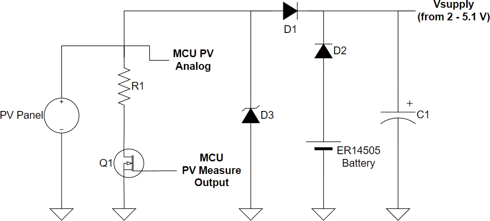
The sensors’ data collection system was based around the Rock- etScream Mini Ultra™ Arduino-compatible microcontroller, a low- power specialty microcontroller based on the Arduino ATmega4808, which used a sensing resistor and its built-in voltage sensor to record the PV panel voltage and translate it into irradiance measurements. For energy storage, the sensors used a 4.7-farad supercapacitor as well as a non-rechargeable 3.6-volt lithium thionyl chloride battery for use during times when PV power was not available. A circuit diagram for the sensors in shown in Figure 1 and an exhaustive list of the materials used in the sensor design is presented in Table 1.
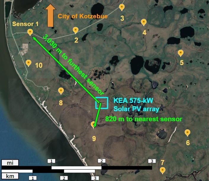
In total, ten sensors were constructed and deployed in an ap- proximately circular pattern around the 575-kW eastern portion of the KEA PV array. The locations of the sensors were selected based on the minimum distance required to detect a ramp event caused by a cloud 2 minutes before the event would impact the PV array. This was calculated by using historical wind speed data from the site as a surrogate for cloud speed. A cloud moving at the 99.9th percentile wind speed (21.1 m/s) would require a distance of approximately 2500 m to meet the desired 2-minute delay, so each sensor was placed as close to 2500 m from the PV array as possible given the physical accessibility of the site as well as local land use agreements. The locations of the ten sensors in reference to the KEA 575-kW PV array are shown in Figure 2.
3.1.1. Data Transmission and Limitations
Cellular modems are commonly employed for similar remote data collection tasks, however the extremely limited cellular coverage in the area surrounding the KEA PV array made this an infeasible option. While satellite communications do not have this geographic restriction, the high cost and power consumption of satellite modems would have necessitated a much more expensive and cumbersome sensor design. For these reasons, this study made use of short-range radio transmissions using the Long-Range Wide Area Network (Lo- RaWAN) protocol [27]. LoRaWAN uses a system of centralized nodes, often called “gateways,” which serve as connection points between LoRaWAN-capable devices and the wider internet. For this study, one Dragino™ LG16 Indoor LoRaWAN gateway was installed at the KEA PV site (where a wired internet connection was available) and was fitted with a Dragino™ ABL-AN-040 fiber- glass extended-range outdoor antenna for improved signal reception. The sensors themselves each utilized a Seeed Grove™ LoRa-E5 LoRaWAN module to interface with the gateway and transmit data.
While the LoRaWAN protocol does generally require much less power than competing technologies, transmitting data still ac- counted for the vast majority of energy used by the sensors. To ensure a reasonable service life of at least 2 years, limits were placed on the frequency of data collection and transmission. The sensors were programmed to record and store a rolling window of 10 irradiance measurements, each 2 seconds apart but only transmit- ted the 10 data points currently in memory when certain threshold values were met:
- Absolute mean difference between the last 10 data points is greater than 6.5 W/m2.
- Absolute median difference between the last 10 data points is greater than 10 W/m2
These values were determined by calculating a sensor’s max- imum average energy usage which would still allow it to operate and transmit data using only its PV panel and supercapacitor during the day. A maximum number of transmissions per day was then calculated from this value and found to be approximately 1 trans- mission every 2 minutes. The maximum measured irradiance ramp rate which would result in an average of 1 ramp every 2 minutes during daylight hours was determined empirically using global hori- zontal irradiance (GHI) data collected from the KEA PV site. The first 10 data points (20 seconds) of each of these qualifying ramp events as well as the mean and median absolute differences between each of the first 10 data points were recorded for each ramp and the averages of these values were used to set the thresholds listed above. Transmissions were also halted entirely when the mean of the 10-measurement window was less than 15 W/m2.
Table 1: Sensor components.
| Component | Manufacturer | Model |
| Microcontroller | RocketScream | Mini Ultra™ |
| LoRaWAN module | Seeed | Grove LoRa-E5 |
| Solar panel | Voltaic Systems | 1 Watt 6 Volt Solar Panel |
| Solar panel mounting bracket | Voltaic Systems | Solar Panel Bracket – Small |
| Solar panel cable extension | Voltaic Systems | Cable Extension with Exposed Leads |
| Supercapacitor (C1) | Eaton | PHV-5R4V474-R |
| Diode (D1, D2) | Diodes Incorporated | 1N5817-T |
| Zener diode (D3) | Vishay General Semiconductor | BZX85B5V1-TR |
| Sensing resistor (R1) | Vishay General Semiconductor | MRS25000C6808FC100 |
| MOSFET transistor | Infineon Technologies | IRLZ44NPBF |
| ER14505 battery | EVE Energy Co. | ER14505 STD |
| Antenna for LoRaWAN module | SparkFun Electronics | 915MHz LoRa Antenna |
| LoRaWAN antenna adapter | Padarsey Electronics | RF U.FL(IPEX/IPX) Mini PCI to SMA Female Pigtail |
| Breadboard (for mounting internal components) | Adafruit | Perma-Proto Quarter-sized Breadboard |
| Cable tension relief glands | Lokman | PG7 |
| Electronics housing | Polycase | An-16F |
| Tripod mounting bracket | Liuhe | Universal Stainless Steel Vertical Pole Mount |
| Mounting tripod | Davis Instruments | Weather Station Mounting Tripod |
As a final precaution against excessive power draw, the sensors were programmed to be unable to transmit more than once in any 2- minute period. This impacted the ultimate quality of the data since, if another ramp event were to occur within that 2-minute waiting period, it would not be recorded. It was ultimately decided that the detection of ramp events large enough to warrant the activation of a diesel generator at a resolution greater than 2 minutes would likely not be significantly more valuable to grid operators, since the generators required to ensure grid stability would already be in the process of starting.
3.2. Data
Data used in this research were sourced from two distinct locations:
(1) the Kotzebue solar PV site and (2) the NREL 1-second Global Horizontal Irradiance Measurement Grid in Oahu, Hawaii.
The data from the Kotzebue site can be broken down into three categories:
- 1-minute resolution alternating current (AC) power produc- tion data measured from the inverter one of eight 72-kW sub-arrays that form the eastern, 575-kW segment of the KEA PV array.
- 1-minute resolution meteorological data recorded from a me- teorological station immediately adjacent to the sub-array.
- 2-second, non-continuous irradiance data from each of the 10
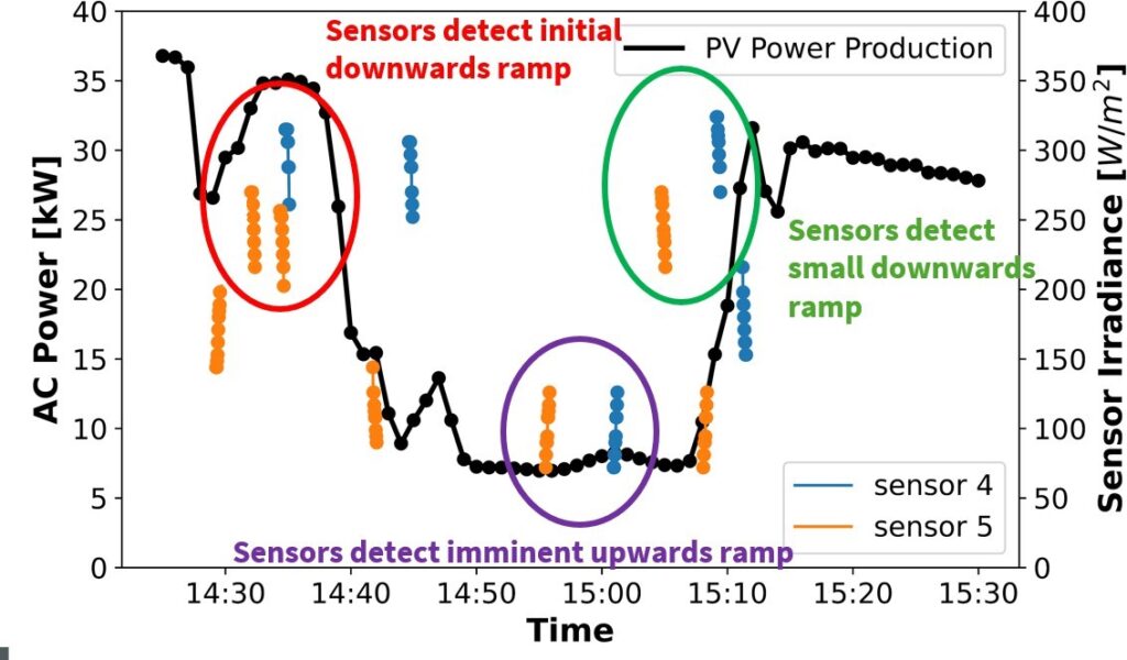
PV and meteorological data at the Kotzebue site were measured every 5 seconds via the same data logger and averaged over each minute at the time of recording, leaving only the 1-minute resolution data available. Figure 3 shows an example period of approximately 70 minutes of AC solar PV power data as well as several ramp events from sensors 4 and 5, demonstrating the difference in tempo- ral resolution and continuity.
Figure 3 shows that, while the sensors were not able to capture the entire irradiance time series, they do transmit clear upwards or downwards ramp event data in the minutes preceding the ramp experienced by the PV array.
Data from the meteorological station and KEA sub-array were collected from late 2021 through March of 2023 with 486 days of data deemed usable. While the sensor network was installed in July of 2022, only 71 days of data between August and November of 2022 were deemed to be usable due to persistent snow cover of the sensors’ 1-watt reference PV panels as well as low light levels during the winter months of the 2022-2023 season.
The 1-Second Global Horizontal Irradiance Grid data set pro- vided by NREL consists of 17 GHI sensors distributed across ap- proximately 1 km2 in Oahu, Hawaii. Data were collected from these sensors from March of 2010 through October of 2011 [28]. A number of studies have used this data set as training data for various solar nowcasting models [20, 26, 29] and it was used in this study to validate the results from the Kotzebue site as well as to investigate the impact of differing ramp rate profiles on the efficacy of various models. The NREL Oahu data set is not a perfect analog to the Kotzebue data set as it lacks wind speed and direction data. Additionally, the sensors were placed much closer together than those deployed in Kotzebue for this study.
Due to the different sample rates between the Oahu and Kotzebue data sets, it was necessary to modify the Oahu data set to simulate the limitations of the Kotzebue sensors. First, the data were resampled to a 2-second resolution to match the internal sampling rate of the Kotzebue sensors then the ramp detection thresholds and 2-minute transmission limit described in Section 3.1 were also applied. This resulted in a discontinuous data set comparable to the Kotzebue sensor data. Additionally, since the Oahu sensor network did not include a centrally located PV array, the center-most sensor was chosen as a surrogate and its data were resampled to a 1-minute resolution to match the data from the KEA PV array.
3.2.1. Quality Control
For the solar PV power production data, the capacity of the sub- array inverter (67 kW) was used as a maximum reference value. All data points exceeding 67 kW were discarded.
Data were also removed based on their associated solar eleva- tion (angle of the sun above the horizon). There is evidence to show that irradiance data with solar elevation angles less than 5◦ can be unreliable due to low incident angles on reference surfaces [30, 31]. In this data set, due to Kotzebue’s extreme latitude, solar elevation did not exceed 5◦ at all from January 1st to January 28th or from November 13th to December 31st but did not overlap with the available data period.
3.2.2. Data Restructuring
Data from the sensors were transmitted at a 2-second resolution with gaps between of at least 2 minutes while data from the PV sub-array and meteorological data were logged as 1-minute averaged data. A truncated example of some of the collated data from a day in September, 2022 is shown in Table 2 below.
Note that data from multiple sensors may overlap but the ma- jority of each sensor column is empty due to the 2-minute trans- mission restriction. Data from the meteorological station and solar PV sub-array (the examples of power production and ambient air temperature are used in Table 2) is only timestamped each minute, leaving substantial data gaps in this unmodified state.
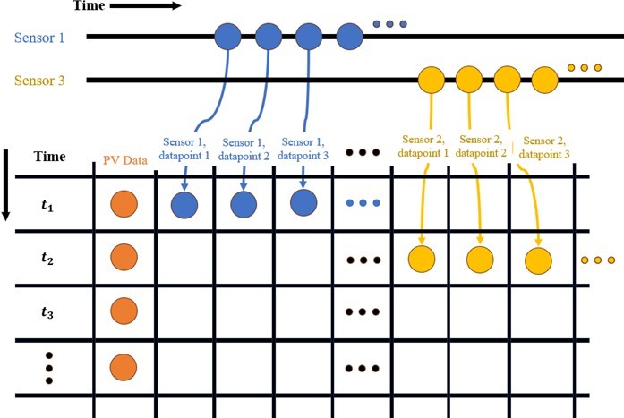
Neural networks of the kind used in this study cannot be trained with missing data, so data manipulation was required to produce a continuous data set. One solution considered was to resample the solar PV sub-array and meteorological data to a 2-second resolution but this proved impractical due to the gaps in the sensor data caused by the 2-minute transmission limit. It was instead decided to alter the sensor data to fit the 1-minute resolution of the remaining data fields. A diagram of this manipulation is shown in Figure 4 below.
The key insight for this manipulation is that, due to the 2-minute hard cap on sensor transmissions, any given minute can only con- tain, at most, one transmission per sensor. This allowed for the sensor data to be pivoted, with each of the 10 data points from each transmission assigned their own column. In this structure, assum- ing an arbitrary sensor transmission is a vector of 10 data points [t1, t2, …, t10], then column ”sensor 1, data point 1” contains every t1 data point from sensor 1, ”sensor 1, data point 2” contains every t2 data point from sensor 1, and so on with column ”sensor m, data point n” containing all nth (1-10) data points from sensor m (1-10).
Table 2: Example of collected data.
| Time | Sensor 1 | Sensor 2 . . . PV Pwr. (kW) | Air Temp. (C) |
| 0:00 | – | – . . . 52.55 | 13.33 |
| 0:10 | 288 | – . . . – | – |
| 0:12 | 225 | – . . . – | – |
| 0:14 | 225 | – . . . – | – |
| 0:16 | 252 | – . . . – | – |
| 0:18 | 243 | – . . . – | – |
| 0:20 | 243 | – . . . – | – |
| 0:22 | 234 | 378 . . . – | – |
| 0:24 | 225 | 387 . . . – | – |
| 0:26 | 225 | 400 . . . – | – |
| 0:28 | 225 | 414 . . . – | – |
| 0:30 | – | 423 . . . – | – |
| 0:32 | – | 432 . . . – | – |
| 0:34 | – | 432 . . . – | – |
| 0:36 | – | 432 . . . – | – |
| 0:38 | – | 387 . . . – | – |
| 0:40 | – | 378 . . . – | – |
| 0:42 | – | – . . . – | – |
| 0:44 | – | – . . . – | – |
| 0:46 | – | – . . . – | – |
| 0:48 | – | – . . . – | – |
| 0:50 | – | – . . . – | – |
| 0:52 | – | – . . . – | – |
| 0:54 | – | – . . . – | – |
| 0:56 | – | – . . . – | – |
| 0:58 | – | – . . . – | – |
| 1:00 | – | – . . . 54.51 | 13.21 |
1 took place during minute 1 while the ramp detected by sensor 3 occurred in minute
2 and was thus assigned accordingly.
To preserve some additional time resolution information, the time from the beginning of the ramp event until the end of its corre- sponding minute was recorded and assigned its own data field for each sensor. To aid the models’ ability to isolate ramp events, a bi- nary flag field was created for each sensor to indicate if that minute contained a transmission (1 for transmission, 0 for no transmission). If a sensor did not transmit a ramp event in a given minute, these fields for that sensor were set to 0.
In total, 125 fields were used as inputs to the models:
- 10 data-point fields for each of the 10 sensors
- 1 time-to-end-of-minute field for each
- 1 ramp-event binary flag for each
- 2 for wind direction sine and cosine
- 1 for wind
- 1 for solar elevation to aid the models in tracking the time of
- 1 for the solar PV
Of the 71 days of available data, 47 were used for training data, 16 were used for validation, and eight days with a notable diversity of ramp profiles were not used in the training process at all and instead selected for testing.
3.3. Solar Variability
Forecasting weather events in general is a difficult task. Solar ir- radiance, and thus PV production, undergoes long-term seasonal variation due to the solar cycle and short-term variability from weather effects such as clouds. Figure 5 shows an example of four different days of measured solar PV AC power production under dramatically different cloud coverage conditions.
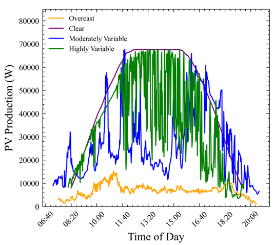
Assessing the variability of solar PV production on both timescales is another common tool apart from deterministic fore- casts to which can help improve PV integration efficiency. While a number of metrics exist for evaluating the variability of time se- ries data, a simple one used often when assessing PV production specifically is the Variability Index (VI) [33]. This metric was used in previous work by these authors in assessing the variability of the Kotzebue PV production data set [32].
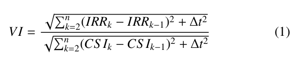
VI characterizes the variability of solar PV data over a given period of n time steps by comparing it to a corresponding clear-sky (synthetic, unobstructed PV data) over the same period. A value of 1 indicates a perfectly clear day while larger values correspond with increasing variability. References [33] and [32] used the VI metric to categorize daily variability over the course of a year. In (1) above, IRRk is the measured irradiance at time step k, CS Ik is the clear-sky irradiance at time step k, n is the number of time steps, and ∆t is the length of time between time steps.
This metric is of particular interest in this work because it pro- vides a potential explanation for the differences in forecasting ac- curacy depending of the data used to train models. As outlined in Section 3.2, a comparison was done between the Kotzebue PV and sensor data and data from the NREL sensor network in Oahu. These two locations have significantly different daily and yearly weather patterns and, since the objective of this research is to develop methodologies for detecting sudden ramp events, it was deemed useful to evaluate the frequency of such events across the two data sets.
3.4. Artificial Neural Networks
Artificial neural networks (ANNs) refer to a wide classification of computational tools which approximate the function of a bi- ological brain. They are composed of complex collections of simple arithmetic operations which can be optimized to produce a desired output from a given input [34]. Because they can be adapted to arbitrary problems, ANNs have found widespread use across many data-driven fields, including solar PV forecasting [35, 36, 37, 38, 39, 40, 41, 42].
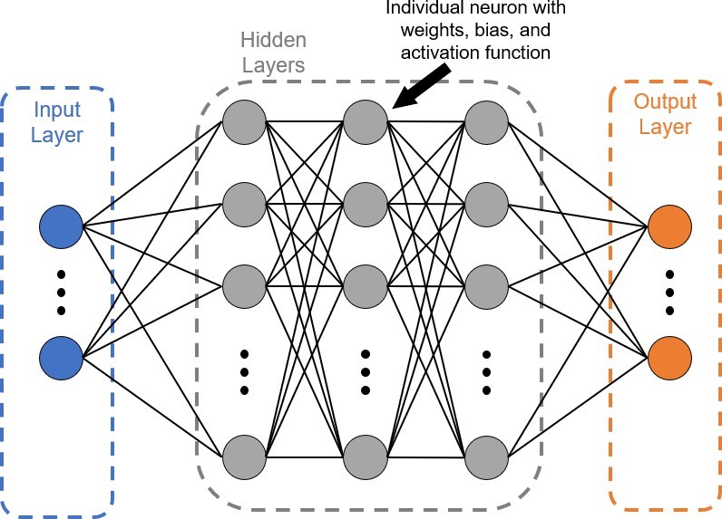
ANNs are composed of interconnected structures called ”neu- rons” which intake the weighted sum of arbitrary numerical inputs, add an arbitrary bias value, and apply a activation function (usu- ally a function bounding between 0 and 1 or restricting to positive values). The output y of a neuron with n inputs can be written as y = f (X · W + b) where X is the vector of input values to the neuron [x1, x2, x3, …, xn], W is the vector of weights associated with each of the input values [w1, w2, w3, …, wn], b is the bias, and f is the activation function.
The values which a neuron intakes can either be raw input data such as temperature, wind speed, etc. or the output of another neu- ron. The ability to stack neurons into layers gives ANNs the ability to model complex tasks efficiently [43]. The layers of neurons be- tween the input and output layers are often called ”hidden layers” as their inputs and outputs are not directly captured. Figure 6 below shows a diagram of an arbitrary ANN with its interconnected layers. For solar PV forecasting, examples of input fields might include am- bient temperature, time-of-day, current solar irradiance, etc. while the output layer would necessarily be future PV production.
ANNs are optimized to learn input/output relationships in a given data set through a process called ”training” during which the weights and bias of each neuron are iteratively adjusted until a stable solution is found. Training is performed through a process called ”backpropagation” where, starting from the output end of the network, a gradient descent algorithm is used to find the value of each weight and bias for which some user-defined error function is minimized [44]. This procedure uses a loss function Q(w) of the form:
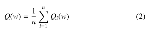
where n is the length of the data set and w is the weight or bias value to be optimized. An initial guess for w is selected then iteratively updated using the process: w = w − α∇Q(w) where α is a scalar factor often called the ”learning rate” which modulates the size of each step down the gradient and ∇ is the gradient operator. This iteration repeats until w stabilizes at some minimum value of Q(w), at which point the next weight or bias is adjusted. This repeats until the entire network is optimized [45].
3.4.1. Long Short-Term Memory
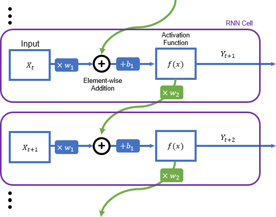
While the general ANN structure (sometimes called a dense ANN, since each neuron is connected to every neuron in the next layer) is still widely used for numerous forecasting applications, other vari- ants exist which are specialized for specific tasks. One such variant is the RNN which is designed for sequential applications, such as time series forecasting. RNNs work by adding the weighted output of each neuron’s activation function together with the weighted input from the next time step. Each neuron can be thought of as a chain of ”cells” which each share the same weights and biases. Figure 7 below shows the structure of a simple RNN neuron [46].
Since each cell in the chain shares weights and a bias, an RNN which intakes n time steps will have its output values scaled by wn. For even small values of n, this can quickly lead to an unstable gradient and is often referred to as the ”exploding/vanishing gra- dient problem.” This flaw makes simple RNN structures like that shown in Figure 7 unfeasible for learning the longer-term, yearly dependencies required for accurately forecasting solar PV data [47].
LSTM-based models have become an extremely popular choice for time series forecasting due to its ability to overcome the explod- ing/vanishing gradient problem [48, 49, 50]. This is achieved by a more complex cell structure which contains three sub-units called ”gates,” each of which contains either one or two sets of their own weights, biases, and activation functions. This structure allows the LSTM cell to maintain two internal states: the short-term and long-term memory. The short-term memory retains information about the previous time steps in the chain while the long-term memory is used to learn dependencies across much wider timescales, allowing long-term pattern information to be transferred without the gradient growing too large/small [51, 52]. The structure of an LSTM cell can be seen in Figure 8 below.
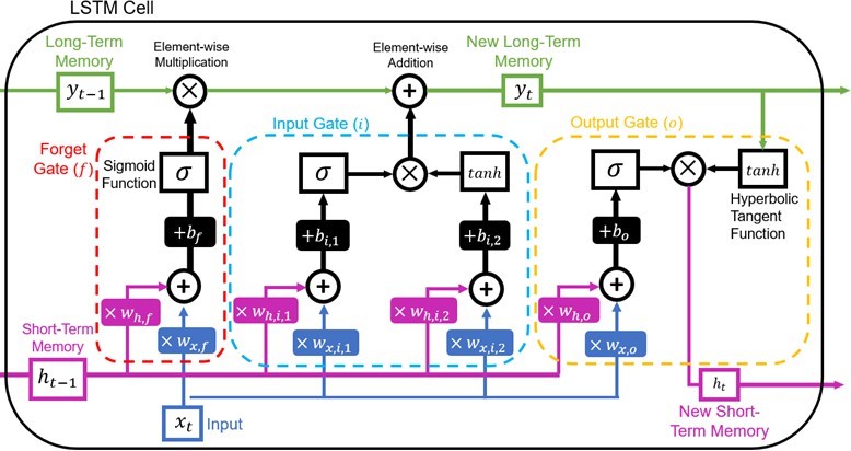
The output of the three gates at time t can be expressed as follows:
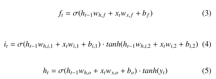
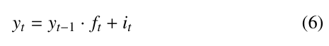
Here, xt can either be a scalar (in the case of a single variable in- put) or a vector of length equal to the number of input variables and the weights w and biases b are the same shape as xt. All operations are also assumed to be element-wise across the vector. The current timestamp’s long-term memory state, yt, can be expressed as:
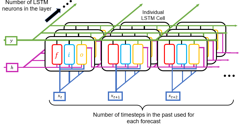
Like with simple RNNs, the weights and biases inside each LSTM cell are shared between all cells in the neuron’s chain. LSTM cells can also be interconnected into layers, processing multiple time steps simultaneously, and allowing for even deeper pattern recogni- tion (see Figure 9 below).
3.4.2. Gated Recurrent Unit
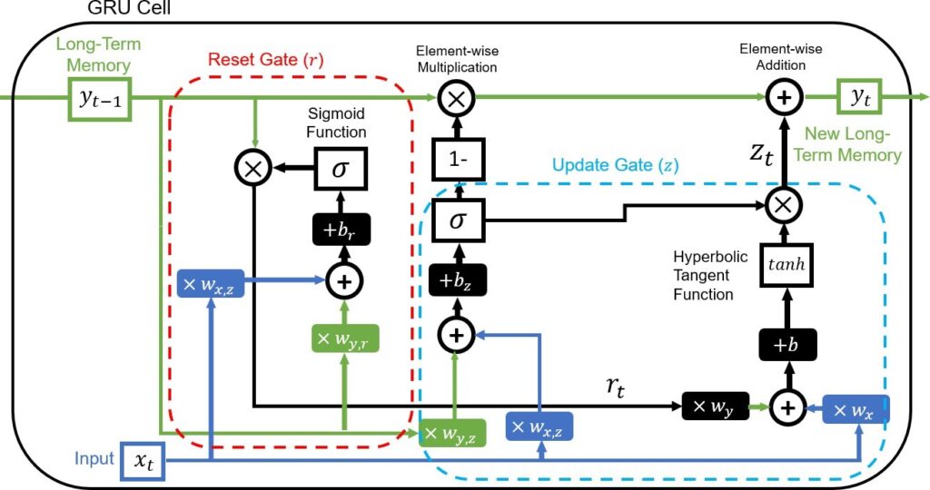
The Gated Recurrent Unit (GRU) model is an advancement on the LSTM and is fundamentally very similar in its application with some notable differences. As opposed to the three gates present in the LSTM cell, GRU cells only have two. Additionally, the GRU design opts to forgo the two separate memory states of the LSTM in favor of one, long-term memory [53, 54]. The structure of the GRU cell is shown in Figure 10.
Here, the output states of the reset and update gates can be expressed as:
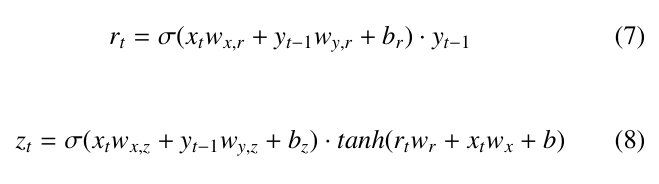
Finally, the new singular long-term state, yt can be written as:

This highlights the fundamental differences between the LSTM and GRU models, primarily the fact that the GRU model cannot con- trol the amount the previous long-term state yt−1 to intake into the current calculation (which LSTM is able to do with the forget gate). This potentially allows for a more nuanced ability to learn across multiple time steps. There is also the lack of short-term memory state in the GRU formulation. This affords the model notably more computational efficiency, allowing for larger models to be practical while also potentially limiting its ability to extract more detailed patterns from training data [55].
3.4.3. 1-Dimensional Convolutional
Convolutional Neural Networks (CNNs) are a subset of ANNs most commonly used in the field of image processing. They use a 2- dimensional sliding window over a data set and then feeding that window into a set of connected neurons. This same methodology can be applied, with some adjustment, to 1-dimensional sequential data, such as a time series. These 1-dimensional CNNs are often referred to as Conv1D models when used in this context. Conv1D models are particularly useful for reducing the number of input variables in large, multivariate time series as well as for determining which patterns and combinations of variables have the largest im- pact of accuracy. As mentioned in Section 2, they are often layered before LSTM and/or GRU layers in order to reduce the input size and improve training efficiency [56]. The structure of a Conv1D neuron is shown
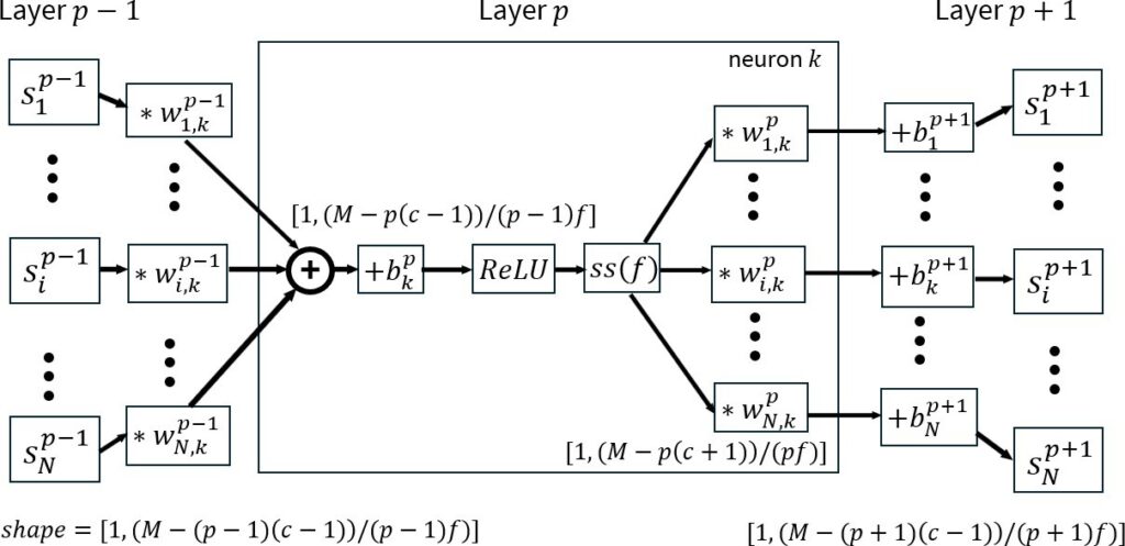
Figure 11 shows the Conv1D data flow process over a data set with N data columns and an initial window of size M. The output vectors of the previous layer, sp−1 convoluted (∗ being the convo- lution operator) with ”kernels” or vectors of shape [1, c] (denoted by wp−1). These resulting vectors are now reduced in size by c − 1, since the kernel must fit entirely within the rolling window M. A bias bp is then applied followed by a rectified linear unit (ReLU) activation function. The vector is then sub-sampled (denoted by the ss operator) by a factor of f before being convoluted with the kernels of layer p and interconnected with the neurons of layer p + 1. The output of layer p for each data column i can be expressed as:
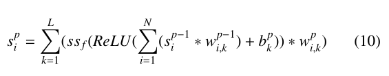
where L is the number of neurons in layer p and each subsequent layer reduces the vector size, thus limiting the possible combinations of kernel and window size [57].
3.5. Model Structures and Implementation
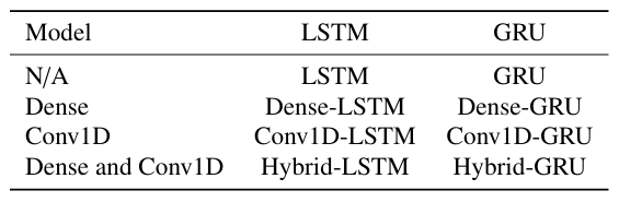
For this study, eight combinations of LSTM, GRU, Conv1D, and Dense layers were tested. These include: a base LSTM and GRU model, an LSTM and GRU model proceeded by a Dense model, an LSTM and GRU model preceded by a Conv1D model, and a ”hybrid” model, which combines the Conv1D, LSTM/GRU, and Dense models. The naming convention for these eight models is presented in Table 3 below.
Table 3: Base model structure naming conventions.
Another useful addition to machine learning models is the ”dropout” layer. Not a computational layer like the Conv1D, Dense, or CNN layers, the dropout instead randomly sets a specified fraction of the weights between connected layers in a model to zero on each training iteration. This is highly valuable to combat a phe- nomenon known as ”overfitting” whereby a model will optimize its weights and biases to fit its training data set but will perform poorly on an as-yet unseen (or ”validation”) data set. This happens because the model learns patterns which are specific to the training data but cannot be generalized to future data. The dropout layer forces the model to adapt to variation in the input data set as, with the dropout layer, the model now cannot rely on any one neural pathway be- tween layers. The generalized model structure with dropout layers is shown in Figure 12. The specific number of Conv1D, LSTM/GRU and Dense layers, as well as the fraction of each dropout layer, is specified in Section 3.7 below.

These eight models were constructed, trained, tuned, and val- idated using the Python library ”Keras” which provides a wide variety of tools for implementing machine learning models of all kinds including neural networks. Keras provides a framework for creating hybrid neural networks in a highly modular fashion and is ideal for quickly prototyping models while also including a robust system for refining and validating model performance.
3.6. Performance Metrics
The metrics used to evaluate the efficacy of the various model struc- tures were divided into two categories: (1) standard error metrics and (2) event-based metrics.
3.6.1. Standard Error Metrics
Previous research into solar PV forecasting across all time hori- zons used some combination of the standard statistical error metrics MAE, MSE, RMSE, and the coefficient of determination, r2.
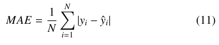
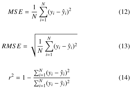
In the above equations, y is the actual data set, yˆ is the forecast, y¯ is the mean of the actual data set, and N is the length of both y and yˆ. Each of these metrics quantifies the error of a forecast differently. MAE treats all individual errors proportionally while MSE penalized larger absolute differences more severely. RMSE preserves the units of the input data and is also used to calculate another metric (”skill”), which is discussed below. r2 is bounded between 0 and 1 and shows the degree to which changes in yˆ are determined by changed in y. In order to more directly compare results with previous work, variants of MAE and MSE, normalized Mean Absolute Error (nMAE) and normalized Mean Square Error (nMSE) were used. These simply scale the error by the maximum value of the actual data set.
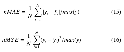
Forecast skill compares the RMSE score of yˆ to that of a per- sistence model. A persistence model, sometimes referred to as a ”naive” model, is the simplest prediction algorithm possible. It simply assumes that the next data point will be the same as the previously measured data point.
![]()
In (17), H is the forecast horizon, or the number of steps ahead to be forecast. The most commonly used skill definition uses RMSE as its metric.
A score of 0 indicates that the model in question performed no better than a persistence model while negative and positive scores demon- strate worse and better relative performance respectively. While not itself useful for generating meaningful forecasts, persistence models and forecast skill are important tools for establishing baseline model performance. Data sets with large periods of little change, such as extremely sunny or extremely overcast days in the case of solar irradiance data, can lead to surprisingly good performance from a persistence model in terms of the standard error metrics.
3.6.2. Event-based Metrics
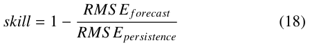
While the standard error metrics are useful for understanding the aggregate performance of a model, the ultimate goal of this research is to develop a deterministic forecasting method which can accurately predict individual large ramp events which would threaten the stability of a high-solar-penetration electric grid. In order to more directly measure this capability, the models presented in this paper were also evaluated on an individual event basis. This was accomplished using three standard event-based metrics: Precision (PR),Recall(RE),andFβ.
Hits, misses, and false alarms are binary classifications of data points. PR represents a model’s ability to only forecast events which actually happen while RE reflects its success at actually forecasting events in the first place. In (21), β is a scaling factor used to weight PR and RE differently. These metrics are commonly used in ma- chine learning classification applications, but are rarely applied to time series forecasting. This makes sense for situations in which one is primarily concerned with cumulative performance but, con- sidering the highly event-based nature of this research, these metrics were warranted. Additionally, while it may be that those using such a model would place more importance on either PR or RE in their calculation of Fβ, this research evaluated all models at β = 1, which is written as F1.
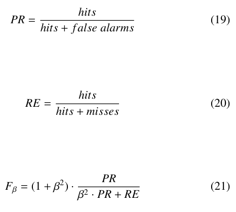
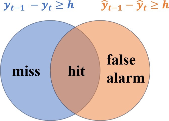
Applying these metrics to a time series data set first required defining hits, misses, and false alarms. Since all ramp events are relative, it was necessary to define a minimum ramp size threshold h. Additionally, while both upward and downward ramp events effect grid stability, upwards ramps can be dealt with more easily through dispatchable loads. For this reason, only downward ramp events were considered in this paper. Misses were calculated by first locating points at time t in the actual data set y where yt−1 − yt ≥ h and then evaluating against the forecasted data set yˆ to find if yˆt − yt ≥ h. False alarms were calculated in the opposite way, where all of the data points in the forecasted data set yˆ where yˆt−1 − yˆt ≥ h and then checking if yt − yˆt ≥ h. A hit was defined as a data point for which both yˆt−1 − yˆt ≥ h and yt−1 − yt ≥ h. Figure 13 shows a visual representation of how each event is classified.
Under real-world conditions, the minimum downward ramp magnitude for which a forecast would be useful to a grid operator is extremely dependent on both their specific grid’s configuration and current state. A small grid on a clear day with a large proportion of its power coming from solar PV is able to absorb a different relative ramp magnitude compared to a larger grid with battery storage, alternative generation sources, and low PV penetration. For this reason, PR, RE, and F1 were evaluated over a range of h values in order to explore how the models performed at predicting different ramp sizes. Plotting RE, PR, and F1 versus h can give a visual sense of model performance, but it was still deemed useful to select a con- sistent baseline value of h at which to evaluate the models. The 99th percentile downward ramp rate was selected, which corresponded to approximately 25.3% of maximum PV capacity per minute, and is referred to as h99 throughout the paper. Values of RE, PR, and F1 evaluated at h99 are labeled PRh99, REh99, and F1,h99 respectively.
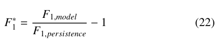
A version of forecast skill to be used with F1 was also devised in order to use a persistence model as a baseline. The F1 forecast skill, F∗ is presented in (22) below and is similar to the standard RMSE definition shown in (18), although modified to preserve the convention of positive values indicating better performance over the persistence model.
3.7. Hyperparameter Tuning
The term ”parameter” is often used to refer to the trainable internal weights and biases within a neural network. Similarly, the term ”hyperparameter” refers to the values which define the overall archi- tecture of the model itself, including the number of layers of each type, the number of neurons (or ”units” as referred to in Keras), and learning rate α. The ideal values for these hyperparameters is highly dependent on the task and there is no set rule for determining them. The model design process often involves significant iterative trial and error where one specifies a range of values for each hyperparam- eter, models are constructed using various combinations of those values, then tested to determine their relative accuracy. This process, often referred to as ”tuning,” is easily automated using Keras. The ranges of the hyperparameters tuned for each type of model layer are presented in Table 4 below.
Table 4: Hyperparameter ranges for each layer.
| Parameter | Min. | Max | Step |
| LSTM/GRU Layers | 1 | 5 | 1 |
| LSTM/GRU Units per Layer | 4 | 128 | 4 |
| Conv1D Layers | 1 | 5 | 1 |
| Conv1D Units per Layer | 4 | 128 | 4 |
| Dense Layers | 1 | 5 | 1 |
| Dense Units per Layer | 4 | 128 | 4 |
| Dropout % Between Layers | 0.0 | 0.3 | 0.05 |
| Learning Rate (α) | 1 × 10⁻⁵ | 1 × 10⁻² | 10 |
The results of the hyperparameter tuning, and thus the architec- tures of the eight models used in this study, are presented in Table 5. The number of values in parentheses denote the number of layers in each category and are listed in order of how the data flows through the layers of the model (i.e. the Dense-GRU model has three GRU layers, the first with 24 units, the second with 24, and the third with 12 a well as 2 Dense layers, the first with 20 units and the second with four). Each layer also has a dropout layer proceeding it, the associated dropout fraction of which is also ordered sequentially in the ”Dropout Layers” column.
4. Results and Discussion
4.1. Performance of the Eight Base Models
Models were constructed using Keras based on the hyperparameter tuning results and each was evaluated using the performance met- rics outlined in Section 3.6. As with the hyperparameter tuning, the loss function used for all eight models was MSE. To eliminate the effect of random variation in the initial parameter guesses during training, each model was trained a total of 10 times, after which all internal parameters were reset. The models were not restricted in terms of how many full passes through the training data, or ”epochs” each training iteration used, but instead a ”patience” threshold was set which automatically ended the training process if three epochs occurred without any improvement in the models’ MSE score. Once trained, each of the 10 iterations of the eight model architectures was used to create a 2-minute-ahead forecast for the eight test days and the performance of the resulting forecasts was evaluated using the standard and event-based metrics. The mean values of the per- formance metrics were calculated across the 10 iterations for each model and are presented in Table 6 below with h99 again equal to 25.3% of maximum PV capacity per minute.
Overall, it is apparent from Table 6 that the standard error met- rics and event based metrics are not strictly linked. The basic LSTM/GRU models performed poorly across all metrics, showing a severe inability to detect ramp events at or above h99 and generally having high error scores across the standard metrics. The Dense- LSTM fared little better, although the Dense-GRU did show the highest PRh99 of any model and improved standard error scores. The Conv1D-LSTM/GRU models displayed particularly interesting re- sults, with the Conv1D-GRU showing underwhelming event-based scores and middling standard errors but the Conv1D-LSTM architecture having a substantially higher F∗1,h99 than any other model,
Table 5: Hyperparameter tuning results.
| Model | RNN Layers | Conv1D Layers | Dense Layers | Dropout Layers | Learning Rate (α) |
| LSTM | (20, 8, 24) | N/A | N/A | (0.15, 0.15, 0.1) | 1 × 10⁻³ |
| GRU | (16, 8, 8) | N/A | N/A | (0.2, 0.2, 0.25) | 1 × 10⁻³ |
| Dense-LSTM | (28, 8) | N/A | (16, 16, 16) | (0.15, 0.15, 0.15, 0.2, 0.2) | 1 × 10⁻³ |
| Dense-GRU | (24, 24, 12) | N/A | (20, 4) | (0.25, 0.1, 0.15, 0.15, 0.15) | 1 × 10⁻³ |
| Conv1D-LSTM | (28, 24) | (36) | N/A | (0.2, 0.1, 0.2) | 1 × 10⁻⁴ |
| Conv1D-GRU | (32, 16, 16) | (64) | N/A | (0.15, 0.2, 0.15, 0.1) | 1 × 10⁻⁴ |
| Hybrid-LSTM | (32, 16) | (36) | (8, 8) | (0.1, 0.1, 0.2, 0.1, 0.15) | 1 × 10⁻⁴ |
| Hybrid-GRU | (28, 4, 20) | (28) | (12, 4) | (0.1, 0.15, 0.15, 0.25, 0.15, 0.2) | 1 × 10⁻⁴ |
Table 6: Model performance across all metrics over the eight test days.
| Model | nMAE | nMSE | r2 | Skill | PRh99 | REh99 | F1,h99 |
F∗ 1,h99 |
| LSTM | 0.215 | 0.412 | 0.825 | -0.165 | 0.000 | 0.000 | 0.000 | -1.000 |
| GRU | 0.211 | 0.370 | 0.843 | -0.104 | 0.000 | 0.000 | 0.000 | -1.000 |
| Dense-LSTM | 0.212 | 0.401 | 0.842 | -0.100 | 0.000 | 0.000 | 0.000 | -1.000 |
| Dense-GRU | 0.181 | 0.331 | 0.869 | 0.000 | 0.895 | 0.009 | 0.017 | -0.630 |
| Conv1D-LSTM | 0.210 | 0.397 | 0.832 | -0.143 | 0.242 | 0.069 | 0.102 | 1.220 |
| Conv1D-GRU | 0.211 | 0.396 | 0.872 | 0.008 | 0.000 | 0.000 | 0.000 | -1.000 |
| Hybrid-LSTM | 0.186 | 0.365 | 0.856 | -0.050 | 0.006 | 0.028 | 0.041 | -0.107 |
| Hybrid-GRU | 0.169 | 0.330 | 0.870 | 0.001 | 0.030 | 0.022 | 0.015 | -0.673 |
although with poor results in other metrics. Finally, the Hybrid- lSTM/GRU models showed improved standard error scores but generally had skill scores around 0, indicating rough parity with persistence models.
The results in Table 6 indicate a rather large gap in performance across the models in terms of the event-based metrics. This was likely due to the relatively small size of the available data set. A downwards ramp event with a magnitude of at least h99 only oc- curred 64 times across the eight test days. This meant that missing only a few more events than another model lead to drastically lower event-based scores. The relative performance of the eight models in terms of F1 is better illustrated in Figure 14.
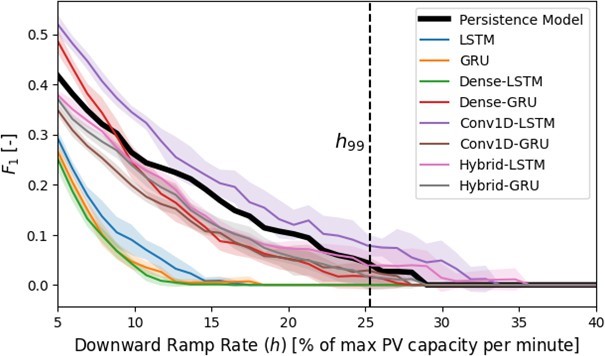
Figure 14 shows the mean and variance of each of the 10 models’ F1 score across the 10 trials along with a persistence model for downwards ramp events h of 5% to 40% of the maximum PV array capacity per minute at increments of 1% with h99 plotted as a refer- ence. No ramp events over 40% per minute were recorded during any of the eight testing days. This plot shows a number of surpris- ing results. The basic LSTM/GRU as well as the Dense-LSTM did not approach the persistence model’s performance for any value of h while the Dense-GRU, Hybrid-LSTM/GRU, and Conv1D-GRU models all performed relatively similarly. Interestingly, the Conv1D- LSTM was able to consistently outperform persistence across all values of h. It is apparent from Figure 14 that there is significant variability within each model’s F1 score, especially for larger values of h where there are fewer ramp events of that size.
The fact that only one of the models was able to barely out- perform the persistence model across multiple values of h shows that these models are struggling to accurately forecasting significant ramp events when they happen. The standard error metrics are also somewhat high compared to similar studies in the literature [10, 20, 58]. One potential reason for the former is the use of MSE as the loss function for the model training process. While MSE does penalize larger errors disproportionately, it does not specifically incentivize models to train in a way which produces good event- based metric scores. This could also be impacted by the hard-coded 2-minute window between sensor transmissions, during which ramp events could be missed. This is most likely due to a general lack of quality training data.
4.2. Comparison to Alternative Data Set
While not the best performing model across all metrics, the Conv1D- LSTM’s notable improvement over other models in terms of F1 warranted further testing. As mentioned in Section 3.2, data from NREL’s Global Horizontal Irradiance Grid sensor network in Oahu, HI was used as a comparison to the Kotzebue PV production data. The same Conv1D-LSTM architecture was used with the 570 days of available data from Oahu, with similar proportions of training, validation, and testing data. This is not an ideal comparison due to the Oahu data set (1) not having associated wind speed and di- rection data, which was an input into the Kotzebue models, and (2) the data from Kotzebue being production data from a PV array compared to the pyranometer measurements from Oahu. Since it takes time for a cloud to move across a PV array, ramp events hap- pen slower when compared to a point-source measurement, like a pyranometer, where the cloud edge impact happens all at once. This spatial smoothing effect has been observed across a wide variety of locations, including Kotzebue [32, 59, 60].
To create a more fair comparison between the Oahu and Kotze- bue data sets, the Conv1D-LSTM model architecture was trained on the same Kotzebue data as before minus the wind speed and direction variables. The models were again fully re-trained a total of 10 times and the results across all metrics were averaged. The F1 plot of these is shown below in Figure 15.
It is apparent in Figure 15 that the Conv1D-LSTM trained on and targeting the Oahu data was much less successful in terms of F1 compared to its respective persistence model but also showed significantly less variance between trials than the Kotzebue Conv1D- LSTM. The lower variance was likely due to the proportionally larger data set from Oahu while the reduced relative performance can likely be explained using the variability index VI outlined in Section 3.3. The daily VI was calculated for both the Kotzebue PV production and the central Oahu PV-surrogate pyranometer. To obtain a better sense of the variability in Kotzebue, 286 days within calendar year 2022 were used. These included the 71 days for which there was also usable sensor array data.
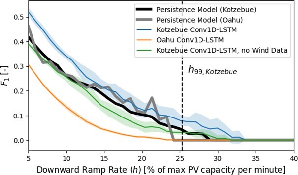
Figure 16 also includes VI values for a plane-of-array (POA) ref- erence cell located at the Kotzebue PV array over the same 286-day time span. This reference cell, like a pyranometer, takes single point measurements and thus should show more variability than the PV array production due to spatial smoothing. This is evident in Figure 16 but it is also clear that the Oahu data set contains significantly more days of higher variability than either of the Kotzebue data sets. This indicates that the increased variability in Oahu is not simply due to a lack of spatial smoothing and is instead a result of local weather patterns.

It is possible that there are so many sudden ramp events in the Oahu data set that a persistence model is able to achieve a rela- tively high F1 score simply because ramp events happen to occur within the 2-minute time horizon of each other very frequently. It is also likely that the Conv1D-LSTM architecture model learned that optimizing for MSE could be achieved without trying to match every local minima/maxima. This is supported by the standard er- ror metrics presented in Table 7 below which show that the Oahu Conv1D-LSTM model performed significantly better than either of the Kotzebue models and even achieved a positive skill.
Table 7: Mean statistical metrics over 10 trials for Kotzebue Conv1D-LSTM and no-wind Conv1D-LSTM models from both Kotzebue and Oahu.
| Model | nMAE | nMSE | r2 | Skill |
| Base Conv1D-LSTM | 0.210 | 0.397 | 0.832 | -0.143 |
| Oahu Conv1D-LSTM | 0.115 | 0.274 | 0.88 | 0.142 |
| No-Wind Kotzebue Conv1D-LSTM | 0.178 | 0.348 | 0.863 | -0.025 |
5. Conclusion
The aim of this research was to develop and test a method for predict- ing sudden ramp events in solar PV production data at a 2-minute time horizon. To this end, a network of 10 solar irradiance sensors was deployed around a utility-scale solar PV array in Kotzebue, Alaska, just above the Arctic Circle. Data from these sensors was used to detect incoming changes caused by passing clouds via a number of deep neural network models, all of which were evalu- ated using both standard error metrics such as MSE, MAE, and forecast skill as well as an application of the event-based metrics PR, RE, and F1. A total of eight models were tested, combining the widely used RNN models LSTM and GRU with 1-dimensional convolutional (Conv1D) and fully connected (dense) networks into various hybrid models. While most of the models showed middling results in terms of the standard error metrics and largely failed to outperform a persistence model in terms of F1 across a range of min- imum ramp magnitudes, the combined Conv1D-LSTM model show notable improvement over the others in the F1 case, although its mediocre standard error metric scores are not enough to definitively conclude that it is the best model for this specific application.
It is likely that a model’s ability to forecast ramp events is re- lated to the frequency and severity of ramp events. When the VI metric was applied to both the Kotzebue and Oahu data sets, it is apparent that the Oahu site experiences significantly more extreme ramp events over a similar time period when compared to the Kotze- bue site. This likely both impedes the models’ ability to accurately learn what constitutes a ramp event as well as gives the persistence models an advantage since shifting the data set by 2 data points is more likely to coincidentally line up with existing ramp events. This performance difference is reflected in the event-based metrics for the Oahu data set as compared to Kotzebue.
There were two notable limitations with this research: (1) the minimum 2-minute window between sensor transmissions, during which time ramp events could be missed, and (2) the general lack of available training data. It is possible that the models were simply unable to reliably learn patterns between the sensor, meteorological, and PV production data sets but would see improved performance with additional data. It is also likely that the failure of most of the models to outperform persistence on an F1 basis was due to the use of MSE (or any standard error metric for that matter) as the loss function. MSE and functions like it are not designed to optimize a model for event-based forecasting. Unfortunately, RE, PR, and F1 use discrete values and as such are non-differentiable, meaning they cannot be used as a loss function.
This research provides two main contributions to the field of so- lar PV nowcasting. For one, it represents by far the highest-latitude deployment of a distributed irradiance sensor network yet tested. It also marks a step forward in evaluating the ability of nowcasting models to accurately and reliably predict sudden changes which might threaten grid stability. While there has been great success in the past two decades in PV forecasting of all kinds according to the standard error metrics, very little analysis has been presented which quantifies the number of critical events captured by models. The few studies which do either evaluate these metrics over too long of a time horizon for this specific application, only evaluate them at one minimum ramp magnitude h, or both [61, 62, 63].
Lastly, assessing the capabilities of artificial intelligence (AI) across various domains has emerged as a vibrant research area. Par- ticularly in the Arctic, AI is proving to be a vital tool for exploring the region’s future and supporting its communities amidst climate change [64, 65]. Further research is essential to fully harness AI’s potential in this context. By evaluating multiple AI models towards Arctic energy challenges, this paper has laid the groundwork for numerous research endeavors in this direction, paving the way for a deeper understanding of AI’s applications in the Arctic and beyond.
Conflict of Interest The authors declare no conflict of interest.
Acknowledgment This work is part of the Arctic Regional Col- laboration for Technology Innovation and Commercialization (ARC- TIC) Program, an initiative supported by the Office of Naval Re- search (ONR) Award #N00014-18-S-B001. This paper is also sup- ported in part by U.S. National Science Foundation’s Major Re- search Instrumentation grant (Award #2320196) and EPSCoR Re- search Infrastructure Improvement Track 4 grant (Award #2327456).
The authors of this paper extend our deepest thanks to the Kikik- tagruk Inupiat Corporation who generously allowed the sensor net- work to be installed on their land, to the Kotzebue Electric Asso- ciation (KEA) for the use of their PV production data, and to the community of Kotzebue as a whole for making this project possible. We also thank Alan Mitchell of Analysis North for his invaluable help in designing the sensors as well as Christopher Pike of the Alaska Center for Energy and Power (University of Alaska Fair- banks) for installing and managing the KEA PV data collection system.
- G. Masson, E. Bosch, A. V. Rechem, M. de l’Epine, “Snapshot of Global PV Markets 2023,” 2023.
- R.-E. Precup, T. Kamal, S. Z. Hassan, editors, Solar Photovoltaic Power Plants: Advanced Control and Optimization Techniques, Power Systems, Springer Singapore, Singapore, 1st edition, 2019, doi:10.1007/978-981-13-6151-7, published: 07 February 2019 (eBook), 20 February 2019 (Hardcover)
- J. Marcos, L. Marroyo, E. Lorenzo, D. Alvira, E. Izco, “Power output fluctuations in large scale pv plants: One year observations with one second resolution and a derived analytic model,” Progress in Photovoltaics: Research and Applications, 19(2), 218–227, 2010, doi:10.1002/pip.1016.
- S. Abdollahy, A. Mammoli, F. Cheng, A. Ellis, J. Johnson, “Distributed compensation of a large intermittent energy resource in a distribution feeder,” in 2013 IEEE PES Innovative Smart Grid Technologies Conference (ISGT), 1–6, 2013, doi:10.1109/ISGT.2013.6497911.
- R. van Haaren, M. Morjaria, V. Fthenakis, “Empirical assessment of shortterm variability from utility-scale solar PV plants,” Progress in Photovoltaics: Research and Applications, 22(5), 548–559, 2012, doi:10.1002/pip.2302.
- H. M. Diagne, P. Lauret, M. David, “Solar irradiation forecasting: state-of-theart and proposition for future developments for small-scale insular grids,” in WREF 2012 – World Renewable Energy Forum, Denver, United States, 2012.
- P. Nikolaidis, A. Poullikkas, “A novel cluster-based spinning reserve dynamic model for wind and PV power reinforcement,” Energy, 234, 121270, 2021, doi:https://doi.org/10.1016/j.energy.2021.121270.
- N. Green, M. Mueller-Stoffels, E. Whitney, “An Alaska case study: Diesel generator technologies,” Journal of Renewable and Sustainable Energy, 9(6), 061701, 2017, doi:10.1063/1.4986585.
- C. S. McCallum, N. Kumar, R. Curry, K. McBride, J. Doran, “Renewable electricity generation for off grid remote communities; Life Cycle Assessment Study in Alaska, USA,” Applied Energy, 299, 117325, 2021, doi: https://doi.org/10.1016/j.apenergy.2021.117325.
- S. Achleitner, A. Kamthe, T. Liu, A. E. Cerpa, “SIPS: Solar Irradiance Prediction System,” in IPSN-14 Proceedings of the 13th International Symposium on Information Processing in Sensor Networks, 225–236, 2014, doi: 10.1109/IPSN.2014.6846755.
- A. Hussain, V.-H. Bui, H.-M. Kim, “Microgrids as a resilience resource and strategies used by microgrids for enhancing resilience,” Applied energy, 240, 56–72, 2019, doi:10.1016/j.apenergy.2019.02.055.
- A. Lagrange, M. de Sim´on-Mart´ın, A. Gonz´alez-Mart´ınez, S. Bracco, E. Rosales-Asensio, “Sustainable microgrids with energy storage as a means to increase power resilience in critical facilities: An application to a hospital,” International Journal of Electrical Power & Energy Systems, 119, 105865, 2020, doi:10.1016/j.ijepes.2020.105865.
- D. S. Kumar, G. M. Yagli, M. Kashyap, D. Srinivasan, “Solar irradiance resource and forecasting: a comprehensive review,” IET Renewable Power Generation, 14(10), 1641–1656, 2020, doi:10.1049/iet-rpg.2019.1227. www.astesj.com 26 H. Toal et al., / Advances in Science, Technology and Engineering Systems Journal Vol. 9, No. 3, 12-28 (2024)
- P. Sukiˇc, G. ˇStumberger, “Intra-minute cloud passing forecasting based on a low cost IoT sensor—A solution for smoothing the output power of PV power plants,” Sensors, 17(5), 1116, 2017, doi:10.3390/s17051116.
- V. P. Lonij, A. E. Brooks, A. D. Cronin, M. Leuthold, K. Koch, “Intra-hour forecasts of solar power production using measurements from a network of irradiance sensors,” Solar energy, 97, 58–66, 2013, doi:10.1016/j.solener.2013. 08.002.
- J. L. Bosch, J. Kleissl, “Cloud motion vectors from a network of ground sensors in a solar power plant,” Solar Energy, 95, 13–20, 2013, doi:10.1016/j.solener. 2013.05.027.
- R. H. Inman, H. T. Pedro, C. F. Coimbra, “Solar forecasting methods for renewable energy integration,” Progress in Energy and Combustion Science, 39(6), 535–576, 2013, doi:10.1016/j.pecs.2013.06.002.
- C. W. Chow, B. Urquhart, M. Lave, A. Dominguez, J. Kleissl, J. Shields, B. Washom, “Intra-hour forecasting with a total sky imager at the UC San Diego solar energy testbed,” Solar Energy, 85(11), 2881–2893, 2011, doi: 10.1016/j.solener.2011.08.025.
- R. Marquez, C. F. Coimbra, “Intra-hour DNI forecasting based on cloud tracking image analysis,” Solar Energy, 91, 327–336, 2013, doi:10.1016/j.solener. 2012.09.018.
- D. Yang, Z. Ye, L. H. I. Lim, Z. Dong, “Very short term irradiance forecasting using the lasso,” Solar Energy, 114, 314–326, 2015, doi:10.1016/j.solener.2015. 01.016.
- M. Jaihuni, J. K. Basak, F. Khan, F. G. Okyere, T. Sihalath, A. Bhujel, J. Park, D. H. Lee, H. T. Kim, “A novel recurrent neural network approach in forecasting short term solar irradiance,” ISA Transactions, 121, 63–74, 2022, doi:https://doi.org/10.1016/j.isatra.2021.03.043.
- P. Kumari, D. Toshniwal, “Deep learning models for solar irradiance forecasting: A comprehensive review,” Journal of Cleaner Production, 318, 128566, 2021, doi:10.1016/j.jclepro.2021.128566.
- S. Mishra, P. Palanisamy, “An Integrated Multi-Time-Scale Modeling for Solar Irradiance Forecasting Using Deep Learning,” CoRR, abs/1905.02616, 2019.
- A. Mellit, A. M. Pavan, V. Lughi, “Deep learning neural networks for shortterm photovoltaic power forecasting,” Renewable Energy, 172, 276–288, 2021, doi:10.1016/j.renene. 2021.02.166.
- A. Bhatt, W. Ongsakul, J. G. Singh, et al., “Sliding window approach with first-order differencing for very short-term solar irradiance forecasting using deep learning models,” Sustainable Energy Technologies and Assessments, 50, 101864, 2022, doi:10.1016/j.seta. 2021.101864.
- X. Jiao, X. Li, D. Lin, W. Xiao, “A graph neural network based deep learning predictor for spatio-temporal group solar irradiance forecasting,” IEEE Transactions on Industrial Informatics, 18(9), 6142–6149, 2022, doi: 10.1109/TII.2021.3133289.
- J. Haxhibeqiri, E. De Poorter, I. Moerman, J. Hoebeke, “A survey of Lo- RaWAN for IoT: From technology to application,” Sensors, 18(11), 3995, 2018, doi:10.3390/s18113995.
- M. Sengupta, A. Andreas, “Oahu solar measurement grid (1-year archive): 1-second solar irradiance; Oahu, Hawaii (data),” 2010.
- A. W. Aryaputera, D. Yang, L. Zhao, W. M. Walsh, “Very short-term irradiance forecasting at unobserved locations using spatio-temporal kriging,” Solar Energy, 122, 1266–1278, 2015, doi:10.1016/j. solener.2015.10.023.
- J. S. Stein, C. W. Hansen, M. J. Reno, “Global horizontal irradiance clear sky models: implementation and analysis.” Technical report, Sandia National Laboratories (SNL), Albuquerque, NM, and Livermore, CA, 2012.
- V. Lara-Fanego, J. Ruiz-Arias, D. Pozo-V´azquez, F. Santos-Alamillos, J. Tovar- Pescador, “Evaluation of the WRF model solar irradiance forecasts in Andalusia (southern Spain),” Solar Energy, 86(8), 2200–2217, 2012, doi: 10.1016/j.solener.2011.02.014.
- H. Toal, A. K. Das, “Variability and Trend Analysis of a Grid-Scale Solar Photovoltaic Array above the Arctic Circle,” in 2023 IEEE 24th International Conference on Information Reuse and Integration for Data Science (IRI), 242–247, 2023, doi:10.1109/IRI58017.2023.00049.
- J. Stein, C. Hansen, M. J. Reno, “The variability index: A new and novel metric for quantifying irradiance and PV output variability.” Technical report, Sandia National Laboratories (SNL), Albuquerque, NM, and Livermore, CA, 2012.
- B. Yegnanarayana, Artificial neural networks, PHI Learning Pvt. Ltd., 2009.
- V. Z. Antonopoulos, D. M. Papamichail, V. G. Aschonitis, A. V. Antonopoulos, “Solar radiation estimation methods using ANN and empirical models,” Computers and Electronics in Agriculture, 160, 160–167, 2019, doi: 10.1016/j.compag.2019.03.022.
- V. Srikrishnan, G. S. Young, L. T. Witmer, J. R. Brownson, “Using multipyranometer arrays and neural networks to estimate direct normal irradiance,” Solar Energy, 119, 531–542, 2015, doi:10.1016/j. solener.2015.06.004.
- F.-V. Gutierrez-Corea, M.-A. Manso-Callejo, M.-P. Moreno-Regidor, M.-T. Manrique-Sancho, “Forecasting short-term solar irradiance based on artificial neural networks and data from neighboring meteorological stations,” Solar Energy, 134, 119–131, 2016, doi: 10.1016/j.solener.2016.04.020.
- H. T. Pedro, C. F. Coimbra, “Assessment of forecasting techniques for solar power production with no exogenous inputs,” Solar Energy, 86(7), 2017–2028, 2012, doi:10.1016/j.solener.2012.04.004.
- S. Z. Hassan, H. Li, T. Kamal, M. Nadarajah, F. Mehmood, “Fuzzy embedded MPPT modeling and control of PV system in a hybrid power system,” in 2016 International Conference on Emerging Technologies (ICET), 1–6, 2016, doi:10.1109/ICET.2016.7813236.
- A. Abbas, N. Mughees, A. Mughees, A. Mughees, S. Yousaf, S. Z. Hassan, F. Sohail, H. Rehman, T. Kamal, M. A. Khan, “Maximum Power Harvesting using Fuzzy Logic MPPT Controller,” in 2020 IEEE 23rd International Multitopic Conference (INMIC), 1–6, 2020, doi:10.1109/INMIC50486.2020.9318188.
- S. Z. Hassan, H. Li, T. Kamal, U. Arifo˘glu, S. Mumtaz, L. Khan, “Neuro-Fuzzy Wavelet Based Adaptive MPPT Algorithm for Photovoltaic Systems,” Energies, 10(3), 2017, doi:10.3390/en10030394.
- S. Mumtaz, S. Ahmad, L. Khan, S. Ali, T. Kamal, S. Z. Hassan, “Adaptive Feedback Linearization Based NeuroFuzzy Maximum Power Point Tracking for a Photovoltaic System,” Energies, 11(3), 2018, doi:10.3390/en11030606.
- C. M. Bishop, Neural networks for pattern recognition, Oxford university press, 1995.
- A. Goh, “Back-propagation neural networks for modeling complex systems,” Artificial Intelligence in Engineering, 9(3), 143–151, 1995, doi: 10.1016/0954-1810(94)00011-S.
- P. Baldi, “Gradient descent learning algorithm overview: A general dynamical systems perspective,” IEEE Transactions on neural networks, 6(1), 182–195, 1995, doi:10.1109/72.363438.
- I. Sutskever, J. Martens, G. E. Hinton, “Generating text with recurrent neural networks,” in Proceedings of the 28th international conference on machine learning (ICML-11), 1017–1024, 2011.
- Y. Bengio, P. Simard, P. Frasconi, “Learning long-term dependencies with gradient descent is difficult,” IEEE transactions on neural networks, 5(2), 157–166, 1994, doi:10.1109/72.279181.
- S. Siami-Namini, N. Tavakoli, A. S. Namin, “The performance of LSTM and BiLSTM in forecasting time series,” in 2019 IEEE International conference on big data (Big Data), 3285–3292, IEEE, 2019, doi:10.1109/BigData47090.2019. 9005997.
- A. Yadav, C. Jha, A. Sharan, “Optimizing LSTM for time series prediction in Indian stock market,” Procedia Computer Science, 167, 2091–2100, 2020, doi:10.1016/j.procs.2020.03.257. www.astesj.com 27 H. Toal et al., / Advances in Science, Technology and Engineering Systems Journal Vol. 9, No. 3, 12-28 (2024)
- X. Qing, Y. Niu, “Hourly day-ahead solar irradiance prediction using weather forecasts by LSTM,” Energy, 148, 461–468, 2018, doi: 10.1016/j.energy.2018. 01.177.
- S. Hochreiter, J. Schmidhuber, “Long Short-Term Memory,” Neural Computation, 9(8), 1735–1780, 1997, doi:10.1162/neco.1997.9.8.1735.
- A. Sherstinsky, “Fundamentals of recurrent neural network (RNN) and long short-term memory (LSTM) network,” Physica D: Nonlinear Phenomena, 404, 132306, 2020, doi:10.1016/j.physd.2019.132306.
- R. Dey, F. M. Salem, “Gate-variants of gated recurrent unit (GRU) neural networks,” in 2017 IEEE 60th international midwest symposium on circuits and systems (MWSCAS), 1597–1600, IEEE, 2017, doi:10.1109/MWSCAS. 2017.8053243.
- R. Zhao, D. Wang, R. Yan, K. Mao, F. Shen, J. Wang, “Machine health monitoring using local feature-based gated recurrent unit networks,” IEEE Transactions on Industrial Electronics, 65(2), 1539–1548, 2018, doi:10.1109/ TIE.2017.2733438.
- J. Chung, C. Gulcehre, K. Cho, Y. Bengio, “Empirical evaluation of gated recurrent neural networks on sequence modeling,” arXiv preprint arXiv:1412.3555,2014.
- S. Kiranyaz, A. Gastli, L. Ben-Brahim, N. Al-Emadi, M. Gabbouj, “Real-time fault detection and identification for MMC using 1-D convolutional neural networks,” IEEE Transactions on Industrial Electronics, 66(11), 8760–8771, 2019, doi:10.1109/TIE.2018.2833045.
- S. Kiranyaz, T. Ince, M. Gabbouj, “Real-time patient-specific ECG classification by 1-D convolutional neural networks,” IEEE transactions on biomedical engineering, 63(3), 664–675, 2016, doi:10.1109/TBME.2015.2468589.
- H. Zhou, Y. Zhang, L. Yang, Q. Liu, K. Yan, Y. Du, “Short-Term Photovoltaic Power Forecasting Based on Long Short Term Memory Neural Network and Attention Mechanism,” IEEE Access, 7, 78063–78074, 2019, doi: 10.1109/ACCESS.2019.2923006
- R. Van Haaren, M. Morjaria, V. Fthenakis, “Empirical assessment of shortterm variability from utility-scale solar PV plants,” Progress in Photovoltaics: Research and Applications, 22(5), 548–559, 2014, doi:10.1002/pip.2302.
- R. Perez, M. David, T. E. Hoff, M. Jamaly, S. Kivalov, J. Kleissl, P. Lauret, M. Perez, et al., “Spatial and temporal variability of solar energy,” Foundations and Trends® in Renewable Energy, 1(1), 1–44, 2016, doi: 10.1561/2700000006.
- M. Abuella, B. Chowdhury, “Forecasting of solar power ramp events: A post-processing approach,” Renewable Energy, 133, 1380–1392, 2019, doi: 10.1016/j.renene.2018.09.005.
- A. Sanfilippo, L. Martin-Pomares, N. Mohandes, D. Perez-Astudillo, D. Bachour, “An adaptive multi-modeling approach to solar nowcasting,” Solar Energy, 125, 77–85, 2016, doi: 10.1016/j.solener.2015.11.041.
- M. Abuella, B. Chowdhury, “Forecasting solar power ramp events using machine learning classification techniques,” in 2018 9th IEEE International Symposium on Power Electronics for Distributed Generation Systems (PEDG), 1–6, IEEE, 2018, doi:10.1109/PEDG.2018.8447599.
- Y. Wang, C. Purev, H. Barndt, H. Toal, J. Kim, L. Underwood, L. Avalo, A. K. Das, “Toward Energy-Efficient Deep Neural Networks for Forest Fire Detection in an Image,” The Geographical Bulletin, 64(2), 13, 2023.
- F. Huettmann, P. Andrews, M. Steiner, A. K. Das, J. Philip, C. Mi, N. Bryans, B. Barker, “A super SDM (species distribution model)‘in the cloud’for better habitat-association inference with a ‘big data’application of the Great Gray Owl for Alaska,” Scientific Reports, 14(1), 7213, 2024, doi:10.1038/ s41598-024-57588-9.
No. of Downloads Per Month