1. Introduction

This study is extension version of the presented conference paper titled “Efficacy of CNN-Bidirectional LSTM Hybrid Model for Network-Based Anomaly Detection” [1] at the 2023 IEEE 13th Symposium on Computer Applications & Industrial Electronics (ISCAIE).

As technology undergoes rapid advancements, the transmission of information has transformed significantly, adopting various methods such as wired, wireless, or guided networks. This evolution in network technology is pivotal to people’s daily activities. Whether it’s communicating with others, accessing online resources, or sharing information, the efficiency and security of these interactions depend heavily on the underlying network infrastructure. A system attains security when it effectively maintains the three essential notions of computer information security: Availability, Integrity, and Confidentiality (CIA). In essence, information security involves safeguarding information from unauthorized entities and protecting against illegal access, use, disclosure, reformation, recording, or destruction of data. Confidentiality guarantees that the information is accessible only to individuals or systems. In information network technology, encryption methods and access controls prevent unauthorized users from gaining access to sensitive data during transmission. Information integrity guarantees that data remains unaltered during transmission. In the context of information network technology, this involves implementing mechanisms to detect and prevent unauthorized modifications to data, ensuring that the information received is the same as what was sent. Availability ensures that information and resources are available and accessible when needed. In an information resources and security environment, availability involves designing robust and reliable systems that can withstand potential disruptions, whether they are due to technical failures or malicious attacks. The overarching goal of information security is to safeguard information from unauthorized access and malicious activities. This includes preventing unauthorized individuals or systems from gaining access to sensitive data, ensuring that information remains unchanged and reliable during transmission, and guaranteeing that information and resources are available when needed.

Measures to achieve information security encompass a range of strategies, including encryption to protect data confidentiality, checksums or digital signatures to ensure data integrity, and redundancy and fault-tolerant systems to enhance availability. Additionally, access controls, firewalls, and intrusion detection are commonly utilized to fortify the security posture of networked systems, mitigating the risks associated with information resources.

A traditional network cannot be fully protected by relying solely on a firewall and antivirus software. These security measures identify predefined anomalous activities and establish the rule to prevent those unusual events by the cyber expert. In anomaly detection, outliers and anomalies are occasionally employed interchangeably. This approach finds extensive use across diverse domains, such as commercial, network attack detection, health systems monitoring, credit card fraud transaction detection, and identifying faults in mission-critical infrastructure systems. Anomaly detection is crucial in cybersecurity, providing robust protection against cyber adversaries. Ensuring safeguard network resources is essential to safeguard the organization from cyber threats.

Anomalies are categorized into point, contextual, and collective types based on the results generated by the detection method [2]. Point anomalies occur when a specific activity diverges from the typical rules or patterns. Contextual anomalies involve unusual patterns within a particular circumstance that consistently differ from numerous normal activities. Collective anomalies occur when a group of related instances exhibit anomalous behavior compared to the normal activity dataset.

          Intrusion detection techniques can be broadly classed into two main types: Signature-based Intrusion Detection System (SIDS) and Anomaly-based Intrusion Detection System (AIDS). Anomaly detections, in contrast, are classified according to their origins, resulting in network-based and host-based intrusion/anomaly detection systems. Detecting anomalies in data is facilitated by employing labels to differentiate between normal and abnormal occurrences. There are three fundamental approaches to detecting anomalies: supervised, semi-unsupervised, and unsupervised methods. In the supervised approach, the system is trained on labeled data, distinguishing between normal and anomalous instances. On the other hand, unsupervised methods detect anomalies without prior labeling, relying on deviations from established patterns. Semi-supervised techniques combine elements of both, using labeled and unlabeled data for training. AIDS overcomes the drawbacks of SIDS by utilizing ML, statistical-based, or knowledge-based methods to model normal behaviors. However, it’s worth noting that anomaly-based detection may produce false results due to alterations in user habits.

Numerous traditional machine learning algorithms favor shallow learning methodologies, giving significant importance to feature engineering designed for smaller data. The feature engineering phase needs more processing time and domain expertise to create pertinent features and eliminate unrelated ones from anomaly detection algorithms. The effectiveness of anomaly detection is intricately tied to feature engineering and data preprocessing implementation. Traditional machine learning methods, characterized by simplicity, low resource consumption, and subpar performance in areas like vision, language processing, and image translations, underscore the limitations of these approaches.

CNN is predominantly employed for image signals, leveraging its architecture to effectively capture and analyze visual information. Individual neurons play a key role in reducing the dimensionality of the network’s features in the lower layers of a CNN. These neurons are adept at identifying essential small-scale features within the images, including boundaries, corners, and variations in intensity. The CNN network links lower-level features to produce more complicated features in the upper layers, encompassing fundamental shapes, structures, and partial objects. The ultimate layer of the network amalgamates these lower features to generate the output results.

The functioning of a long short-term memory differs from that of a CNN due to its specific design to safeguard long-range info within a sequential order. Unlike CNNs, LSTMs are crafted to remember and store information over extended sequences, avoiding the loss of crucial details. In the case of BLSTM, an additional LSTM layer is incorporated, introducing a reversal in the information flow direction. This architectural enhancement addresses challenges related to vanishing gradients, ensuring more effective training by considering information from both forward and backward directions in the sequence.

Data imbalance, including network anomaly detection, is a common challenge in ML applications. In network traffic anomaly detection, data imbalance refers to the unequal distribution of normal and anomalous instances in the dataset for training the detection model. Anomalies in network traffic are typically rare incidents compared to normal activities, leading to imbalanced data.

The deep learning approach addresses issues found in conventional machine learning. The effectiveness of the deep learning-based anomaly detection algorithm relies on factors such as the NN architecture, #hidden layers, activation functions, batch size, and the number of epochs utilized during DL model testing, training, and validation. The careful selection of these factors, including hyperparameters and the architecture of NN in deep learning, is crucial for enhancing the detection accuracy of network traffic anomaly detection. The essential selection of  ML or DL models overcomes the class imbalance problem. The ensemble method, which combines more different individual models, requires longer training time and consumes more resources. The sampling method generates random data or deletes the random data based on the implemented sampling methods to create the balanced form of the final dataset, which is efficient in dealing with the imbalanced dataset.

2. Literature Review

The rapid increase of information and technology has led to widespread connectivity of numerous end terminals to the internet and networks. Those smart terminals contribute to generating substantial volumes of data, commonly referred to as big data. This huge flood of data is a valuable resource for analysis and insights. Machine learning and deep learning algorithms come into play to extract meaningful information from this vast data pool. The daily growth of big data presents difficulties for conventional machine learning algorithms, necessitating thorough feature extraction and discovery. DL substantially increases anomaly detection and model performance. Nevertheless, the dataset’s attributes and features, hyperparameters in deep neural networks, and the structure of neural networks are pivotal elements that impact the efficacy of identifying anomalies in network-based IDS.

Conventional machine learning strongly relies on intricate and time-consuming feature engineering, often impractical for real-time applications. In the [3] study, the authors proposed an approach for payload classification utilizing CNN and RNN to detect attacks, achieving detection accuracies of 99.36% and 99.98% on the DARPA98 network data, respectively. CNN methods discern specific grouping patterns through convolution around input neighborhoods, while RNN works on sequences by calculating correlations between previous and current states. In another[4] study, class imbalance was handled utilizing a CNN with a Gated Recurrent Unit (GRU) hybrid model. To address the data class imbalance and feature redundancy, they used a hybrid sampling technique that integrates Pearson Correlation Analysis (PCA), repeated edited nearest neighbors, Random Forest (RF), and adaptive synthetic sampling. With the detection accuracies of 99.69%, 86.25%, 99.69%, and 99.65% on the NSL-KDD, UNSW_NB15, and CIC-IDS2017 datasets, respectively, their CNN-GRU model performed better.

The research authors[5] proposed using an Adaptive Synthetic Sampling (ADASYN) technique in a DL-based network intrusion detection system to overcome dataset imbalance. On the NSL-KDD network data, they used an autoencoder to reduce dimensionality. The CNN-BLSTM hybrid DL method obtained the greatest F1 score (89.65%) and accuracy (90.73%). To address problems resulting from data in class imbalance and heterogeneous data distribution across various information sources, the research [6] used convolutional neural networks with federal transfer learning. The UNSW-NB15 multiclass network dataset produced an average detection accuracy was 86.85% for the model.

In [7], the researcher addressed data class imbalance on network datasets: NSL-KDD, KDD99, and UNSW-NB15 datasets using heterogeneous ensemble-assisted ML methods for binary and multi-class network intrusion detection. Using the NSL-KDD dataset, the model showed a 96.2% AUC and a true positive rate (TPR) of 94.5%.

 The authors of  [8]discovered that ML classifier performance increased with the decrease in target classes. Conventional ML approaches, such as Naïve Bayes, Random Forest, J48, Bagging, Adaboost, and BayesianNet, were used to investigate this idea on three network traffic-based intrusion datasets: KDD99, UNSW-NB15, and CIC-IDS2017_Thursday.

In a study [9], the authors suggested a method for achieving network intrusion classification with low computing cost, creating a group of target classes based on the nature of network traffic. They created cluster characteristics for each group using K-means on the KDD99 network dataset, resulting in a detection accuracy of 98.84%. However, the intrusion detection model accuracy for user2root (U2R) is notably low at 21.92%, impacting overall performance. In  [10], authors employed a hybrid method, combining CNN and LSTM, to enhance model classification accuracy, achieving 96.7% and 98.1% on CIC-IDS2017 and NSL-KDD network data, respectively.

 In the study[11], CNN and LSTM combined to create a hybrid model was proposed to enhance network intrusion detection model facilities for advanced metering infrastructure through cross-layer features combination. This method achieved the highest network intrusion detection accuracy of 99.79% on NSL-KDD and 99.95% on KDD Cup99 but with limited user2root (U2R) detection capabilities. Similarly, in [12], authors employed a hybrid method of combining CNN and LSTM to improve model network intrusion detection by capturing additional network traffic data’s spatial and temporal features.

In[13], the researchers implemented a hybrid technique based on the mean control of the CNN and BLSTM to address issues of conventional data pre-processing and imbalanced numerical distribution of class instances in the NSL-KDD, achieving the optimal detection accuracy of 99.10%. However, the accuracy for the minority traffic data class remains suboptimal. Using a different methodology, the authors[14] created a DL model that combined CNN and BLSTM to learn temporal and spatial characteristics. Accuracy levels on the binary class UNSW-NB15 were 93.84% and binary NSL-KDD of 99.30%.

Data was preprocessed using one-hot encoding and min-max normalization by authors in [15], which achieved an accuracy of 96.3% on CNN and Bi-LSTM hybrid methods on the multiclass NSL-KDD dataset. Using preprocessed on given NSL-KDD data, researchers in[16] applied the hybrid model using CNN and BLSTM algorithm with a 95.4% accuracy rate. A bidirectional LSTM model was used by the authors in their study [17] for the binary NSL-KDD dataset with the highest accuracy of 98.52%. Using a Bidirectional LSTM deep learning model, authors[18] got 99% accuracy on UNSW-NB15 and KDDCUP-99, which is an exceptional achievement. But a lot of the models that are now in use need help effectively identifying uncommon (rare) attack types, especially user2root (U2R) and remote2local (R2L) attacks, which frequently have poorer detection accuracy as compared with other network attack types.

To overcome the difficulties found in the above literature review, authors in [19]presented a Bi-LSTM-based network intrusion detection system on the NSL-KDD dataset, which offered a binary classification accuracy of 94.26%. Furthermore, the authors proposed a Bi-directional GAN-based method [20] for the NSL-KDD and CIC-DDoS2019 datasets. The bidirectional GAN model demonstrated strong performance with an f1 score and detection accuracy of 92.68% and 91.12%, respectively, on the unbalanced NSL-KDD dataset.

In the research study [17] [1], the Authors used the hyperparameters tunning to obtain the best model performance on network intrusion detection datasets, including NSL-KDD and UNSW-NB15. In[21], the Authors implement the BLSTM model combined with random over-sampling strategies, which produces a high anomaly detection accuracy of 99.83% for multiclass imbalance network anomaly datasets NSL-KDD dataset.

The deep learning model discussed in [3]  and [4] overcomes challenges traditional machine learning encounters in anomaly detection. While the CNN standalone model is unsuitable for sequential data preprocessing, and RNN requires complex data preprocessing, this model effectively addresses these issues. Data imbalance problems are tackled in [5], [6], [7], and [8]. Feature engineering emerges as a critical factor in enhancing the accuracy of both ML and DL models. Much research has been conducted on feature engineering, with studies focusing on attribute grouping found in [9],[10],[11],[12]. The BLSTM, which brings together two distinct LSTMs to allow input processing in both directions (from the past to the future and vice versa), is implemented in [13] , [14], [15], [16],[18],[19], [20] to improve the accuracy of network anomaly detection models.

Most of the researchers mentioned above concentrate on enhancing the detection accuracy of conventional or ML DL models and employ ensemble methods for feature engineering to address data imbalance. However, there needs to be more emphasis on exploring hyperparameter selection in DL-based models, determining the train-test split ratio, and defining the architecture of DNN. Some researchers need to elaborate on adopting these values in their studies. Subsequently, this research addressed these limitations in network traffic anomaly detection systems. We experimented using binary and multiclass versions of the UNSW-NB15 and NSL-KDD. Our focus includes investigating the performance comparison between random under-sampling and over-sampling to identify superior methods for imbalanced network data.

The contributions of our research effort in the area of network anomaly detection and imbalanced datasets are listed as:

15. Examining the impact of CNN and BLSTM neural network architecture and performance for binary/multi-class datasets, specifically NSL-KDD and UNSW-NB15.
16. Exploring the model performance of hyperparameters on binary and multi-class network datasets, namely UNSW-NB15 and NSL-KDD.
17. Exploring the enhancement of CNN Bi-LSTM by varying memory elements and numbers of layers of NN.
18. This study’s interest is developing and implementing a CNN Bi-LSTM hybrid model for network anomaly detection, achieving high accuracy rates of 98.27% on NSL-KDD binary data and 99.87% on UNSW-NB15 binary data.
19. Exploring the network anomaly detection model based on CNN Bi-LSTM using UNSW-NB15.
20. Investigating the random sampling methods for imbalanced data with detection accuracy greater than 99.83% for NSL-KDD multiclass data and 99.99% for the UNSW-NB15 multiclass dataset.

The rest of the paper unfolds: Section 3 delineates the system model and individual blocks comprising our CNN Bi-LSTM hybrid approach. Section 4 elucidates the experimental setup, experimental results, and discussion of the findings, and section 5 encapsulates the conclusion of this research.

3. Network Anomaly Detection Model Description

The complete proposed model comprises the following steps:

1. Network traffic-based data collection
2. Data pre-processing and cleaning
3. Training and testing data preparation
4. CNN BLSTM model preparation
5. Train and test model
6. Evaluation of CNN BLSTM model
7. Compare the model and decision-making

The CNN BLSTM-based model’s entire implementation schematic is displayed in Figure 1. The ensuing sections offer a thorough explanation of the approaches mentioned previously. The components of CNN and BLSTM layers and the intricate architecture of neural networks are seen in Figure 2.

3.1.  Network traffic-based data collection

Numerous datasets are accessible for research in network intrusion detection systems. Examples include the KDD Cup99, Kyoto 2006+, NSL-KDD, CICIDS2017, UNSW-NB15, and several others, providing valuable resources for intrusion detection research. During this research, the UNSW-NB15 and  NSL-KDD datasets are specifically employed.

NSL-KDD KDDTrain+ [22] originates from the DARPA KDD99 dataset, with the elimination of noise and undesired data. This dataset encompasses the complete NSL-KDD training set, including labels denoting attack types and difficulty levels. Comprising 41 features, it delineates five different attack classes: “Normal,” “DoS,” “Probe,” “R2L”, and “U2R”.

NSL-KDD represents a refined form of the KDD99 data, free from duplicate records in the training set and the test sets. Each entry in the dataset consists of 42 attributes, with 41 of them related to the input traffic and the final label indicating whether the traffic is normal or abnormal (target). The KDDTrain+ dataset encompasses 125,973 data entries, while the KDDTest+ dataset consists of 22,544 data entries utilized in this research work. Table 1 documents the detailed information regarding the traffic and data information [23].

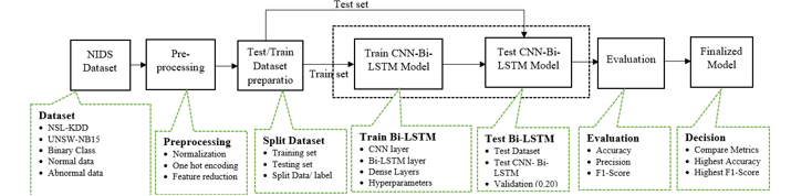
Figure 1: Pipeline for CNN BLSTM hybrid model

Table 1: Details of NSL-KDD data

Traffic	KDDTrain+	KDDTest+
R2L	995	2,885
U2R	52	67
DoS	45,927	7,460
Normal	67,343	9,711
Probe	11,656	2,421
Total	125,973	22,544

                    Similarly, The Australian Centre for Cyber Security (ACCS) cybersecurity research team constructed the UNSW-NB15 dataset [24], unlike KDD99 and NSL-KDD, which is a recently developed network intrusion dataset created by IXIA PerfectStrom tools within the Cyber Range Lab of the ACCS, this dataset consists of approximately 100GB of PCAP files capturing raw network traffic flows between two hosts either server to client or vice versa. The Argus and Bro_IDS tools and 12 other algorithms generated 49 features accompanied by class labels. Numerous records were utilized to construct the training and testing sets, where UNSW_NB15_training-set and UNSW_NB15_testing-set were used during this research work. The training set comprises 175,341 records, while the testing set comprises 82,332 records, encompassing various attacks and normal network activity. Table 2 shows detailed information regarding the attacks and normal traffic.

Table 2: Details of UNSW-NB15 data

Network Traffic	testing-set.csv	training-set.csv
Exploits	11,132	33,393
Generic	18,871	40,000
Worms	44	130
Fuzzers	6,062	18,184
DoS	4,089	12,264
Reconnaissance	3,496	10,491
Analysis	677	2,000
Backdoor	583	1,746
Shellcode	378	1,133
Normal	37,000	56,000
Total	82,332	175,341

      The KDDTrain+ and KDDTest+ subsets of the NSL-KDD dataset were employed in our research experiment—likewise, experiments involved using training-set.csv and testing-set.csv from the UNSW-NB15 dataset.

3.2.  Data pre-processing and cleaning

NSL_KDD data is an improved version of the KDD99 dataset; minimum work is required for data preprocessing. The downloaded separate data files are used to test and train the model. The target class is initially isolated from the training and testing datasets to create the class labels. From the remaining attributes, numerical features and three categorical features—”protocol_type”, “service”, and “flag” are extracted. The categorical features undergo conversion into numerical values using dummy one-hot encoding techniques, while the numerical attributes are standardized using standard Scalar methods. Afterwards, both types of feature sets are combined into a unified data frame, yielding the final data sets for training and testing. One hot encoding generates one binary variable for each individual categorial value. The dummy encoding is similar to one hot encoding and converts the categorical values into numeric binary values. The dummy encoding represents N categories using N-1 binary variable. Let’s say we have three categories of traffic “protocol_type,” “service,” and “flag” that are going to be dummy encoded as [1 0], [0 1], and [0 0], respectively. The standard scalar converts the numeric values so that the data standard deviations become 1.

Since there are different types of services present in the KDDTrain+ dataset and KDDTest+ dataset, the one hot encoding produces unequal numbers of features. The KDDTrain+ dataset contains 126 features, while the KDDTest+ includes a total of 120 features after the implementation of one hot encoding. Those additional features “service_aol,” “service_harvest,” “service_http_2784”, “service_http_8001”, “service_red_i,” and “service_urh_i” are inserted into the KDDTest+ dataset after finding the exact location where those features reside into the KDDTrain+ dataset. We preserved the attacks_types and difficulty_level features because those features are highly relevant to the target class and increase the model’s efficiency.

The UNSW-NB15 dataset was divided into two sets for training and testing purposes: UNSW_NB15_training-set and UNSW_NB15_testing-set. The UNSW_NB15_training-set comprises 175,341 entries, while the UNSW-NB15_testing-set contains 82,332 entries, encompassing various attacks and normal data. Initially, the features on this dataset are 49. First, those categorical attributes are changed into numeric using dummy one hot encoding. All numerical attributes are applied to the standard scalar normalization method. After preprocessing the numeric and categorical features, 192 features for UNSW_NB15_testing-set data and 196 features for UNSW_NB15_training-set data were generated. Again, here we are taking two sets of data: one we can use for training and the other for testing or vice versa. The categorical values of data entries are not the same for both datasets; hence, the one hot encoding produces unequal numbers of features on both data sets after preprocessing.

Some features generated from one hot encoding, such as state_ACC and state_CLO, are not included in the UNSW-NB15_training-set. Similarly, proto_icmp, proto_rtp, state_ECO, state_PAR, state_URN, and state_no features are not included on UNSW_NB15_testing-set. The empty features columns are added in the exact column location of those missing features on the respective dataset, generating 198 features plus one target class.

3.3.  Training and testing data preparation

In experiments concerning the binary NSL-KDD dataset, the training and testing datasets were created using a split ratio. The train-test split approach assesses the performance of machine learning algorithms in making predictions from data that wasn’t part of the training set. We opted for a 70:30 split ratio to generate the train and test dataset. For the CNN BLSTM hybrid model, 70% of KDDTrain+ was used to train, and the remaining data was used to test the model for binary NSL-KDD data.

A similar split percentage was employed in the binary class UNSW-NB15, using the “UNSW_NB15_training-set”. In the case of multiclass experiments for UNSW-NB15 and NSL-KDD, two distinct files were selected—one subset for training the CNN-BLSTM model and another for testing. Detailed information regarding this split is provided in the respective experimental sections.

3.4.  CNN BLSTM model

 CNN is a forward DNN designed for image signal and classification. CNN comprises three primary layers: the convolutional, the pooling, and the fully connected layers. The convolutional layer is the main component of CNN and uses the convolutional operation to grab the various features from the image signal. Then, the number of pooling layers extracts features, and a fully connected layer employs the output from the preceding layer for classification. Combining convolutional layers with pooling layers is responsible for feature extraction, while the final fully connected dense layer is utilized for classification purposes. CNN also involves various hyperparameters, including the number of filters, stride, zero-padding, pooling layers, and others.

An RNN is an artificial NN designed to manage sequential data by integrating feedback loops into its structure. Diverging from conventional feedforward neural networks that linearly handle input data, RNNs feature connections forming loops, enabling them to retain a memory of past inputs and utilize that information to impact the current output. The memory in an RNN serves as a short-term storage, allowing the network to retain information about past events and use it to make predictions about future events. This is especially valuable in applications where context and temporal relationships are essential. Machine learning issues, including speech recognition, language processing, and picture categorization, have been resolved with RNN.

Yet, traditional RNNs encounter challenges, notably needing help with learning long-term dependencies attributed to the vanishing or exploding gradient problem. Advanced RNN versions such as gated recurrent units (GRUs) and long short-term memory (LSTM) networks have been devised in response to these constraints. These architectures include mechanisms for selectively storing and retrieving information across extended sequences, enhancing their effectiveness in tasks that demand capturing long-term dependencies.

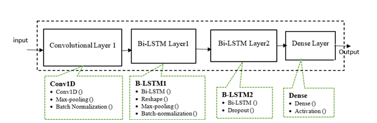
Figure 2: CNN BLSTM layer architecture

LSTM handles the vanishing gradient in RNN. There is a memory block and three multiplicative units in LSTM. The input corresponds to the write operation, output to read and forget gates corresponding to the reset operations for cells that make up the LSTM architecture. By allowing LSTM memory cells to keep and access data for longer periods.  Those multiplicative gates mitigate the vanishing gradient.

To process input in both directions—from the future to the past and from the past to the future—bidirectional RNN combines two independent RNNs. Both forward and backward LSTM networks make up the Bi-LSTM. The features extracted by the forward LSTM hidden layer point forward, whereas those extracted by the reverse LSTM hidden layer point backward. By taking finite sequences into account about earlier and later items, the bidirectional LSTM can anticipate or tag the sequence of each element. Two LSTMs processed in series—one from left to right and the other from right to left—produce this. The CNN and BLSTM hybrid models have several layers, each with a set of hyperparameters. Figure 2 shows the CNN BLSTM’s architectural layout.

3.5.  CNN BLSTM model training

The CNN BLSTM model’s neural network architecture is prepared for training. The datasets consist of two sets: one for training and the other for testing, or vice versa. The split percentage determines how much data is allocated for training and testing when a single data set is present. The selection of hyperparameters for model training is conducted through various experiments involving fine-tuning epochs and batch size to enhance detection efficiency. Within the training data, 20% is designated for validating the CNN Bi-LSTM model.

3.6.  Test the CNN BLSTM hybrid model and evaluation.

Deep learning (DL) and machine learning (ML) models offer performance consistency. After the CNN BLSTM model is built, the model is trained using the training dataset with specified hyperparameter values. These chosen hyperparameter values influence the training duration. Following training, the model can assess the unseen dataset to evaluate its performance. Hyperparameter selection lacks a predefined rule, allowing for random selection and subsequent fine-tuning through various experiments. After the model testing, performance metrics are determined based on the type of ML model employed. In the case of the supervised machine learning model, ground truth values are utilized to measure the performance metrics on the test dataset. Various metrics, such as detection accuracy, precision, F1-Score, recall, program execution time, and Area under the ROC, are available to compare the model efficiency. Confusion metrics from Karas generate True Positive (TP), True Negative (TN), False Positive (FP), and False Negative (FN) values. In the context of a classification report, the terms “weighted” and “macro” refer to different strategies for computing metrics such as precision, recall, and F1-score across multiple classes. Macro-averaging computes the metric for every class separately before averaging them. This means that each class is treated equally in the computation, regardless of size. Macro-averaging gives the same weight to each class, which can be useful when all classes are considered equally. Weighted averaging, on the other hand, takes the average of the metrics, but it weights each class’s contribution based on its proportion in the dataset. In other words, classes with more samples have a greater impact on the average. W weighted averaging is especially helpful when working with unbalanced datasets—where certain classes may have substantially more instances than others.

The classification report provides a thorough summary of the model’s performance metrics for the specified training and testing data sets. Lastly, to assess the performance of our CNN BLSTM hybrid model, the performance metrics are compared with the findings of earlier research publications.

3.7. Compare models and decision-making.

      Several sets of experiments were conducted to find the hyperparameter settings that yielded the best results. Following model testing and evaluation, choosing the best model pipeline from various options is part of the cognitive process of comparison and decision-making. Throughout this study, several sets of experiments are carried out to determine values for various CNN Bi-LSTM model hyperparameters to enhance the model’s performance. To create an effective Bi-LSTM pipeline, it is necessary to decide on the hyperparameters, which include optimizers, number of epochs, batch, NN design, class size, and techniques of raw data preprocessing. This is achieved by evaluating performance metrics across multiple sets of experiments. The performance metrics of the Bi-LSTM model are then juxtaposed with previously published results for the binary/numerous class UNSW-NB15 and NSL-KDD. The class imbalance problem in the multiclass version of both NSL-KDD and UNSW-NB15 datasets was exposed with sampling data during the preprocessing stages. The sampling methods randomly deleted on down-sampling and randomly generated data samples in over-sampling. This resulted in the balanced form of datasets to compare the CNN Bi-LSTM model performance.

4. Results and Discussion

To detect anomalies, intrusion detection uses a mix of DL and ML methods. The implementation of a network anomaly detection model is implied using Python script. Python has specialized packages for building machine learning models, including NumPy, Pandas, Keras, and Scikit-learn. Additionally, commonly used tools like  Java, C#, WEKA, Visual C++, and MATLAB play vital roles in network anomaly detection systems. On the Jupyter Notebook platform, seed values are fixed to guarantee consistency in outcomes over several runs. Plots and tables representing the results of experiments are analyzed using the Microsoft Office suite. Every experiment is run on a Windows machine with an i7 processor and 16GB of RAM.

Python and the packages it is linked with keep version information used in all experiments. For example, TensorFlow 2.9.1, Keras 2.6.0, and Python 3.7.12 are used. Hyperparameters will be determined, performance will be evaluated across class sizes, and the efficacy of various sampling approaches will be assessed about the CNN BLSTM model for the multi-class and binary-class UNSW-NB15 and NSL-KDD. Detailed explanations of these experiments are provided in subsequent sections.

The architecture shown in Figure 2 consists of a single 16-unit convolution layer that uses batch normalization and max-pooling. BLSTM neural network layer 1 contains 50 memory units; batch normalization, max-pooling, and reshaping come next. Bi-LSTM neural network layer 2 with 100 memory units and dropout is also available. The dense layer consists of a sigmoid activation, and the final output is obtained. The detection accuracy of the model is evaluated through a series of tests involving the adjustment of optimizers, learning rate (LR), number of epochs, batch size, and dropout rate. As explained below, the UNSW-NB15 and NSL-KDD binary/multiclass network traffic datasets are used for these investigations.

4.1.  Experiment: Model performance Vs. Optimizers

In the context of ML and DL, an optimizer is an algorithm or method used to adjust the parameters of a model to minimize or maximize a certain objective function. The performance of an optimizer is crucial in training machine learning models because it determines how well the model learns from the data. Choosing the optimizer is essential during the training of the CNN BLSTM model, as it significantly contributes to expediting results for the machine learning/deep learning model.

          TensorFlow offers nine optimizers (Ftrl, Nadam, Adam, Adadelta, Adagrad, gradient descent, Adamax, RMSprop, and  Stochastic Gradient Descent (SGD)) based on the optimizer’s methods. The choice of optimizer can significantly impact the training performance of an ML model. Optimizers may converge at different rates or achieve different final accuracies on a given task. An optimizer’s performance may be influenced by the model’s architecture, the dataset, and the hyperparameters employed.

It is common practice to experiment with several optimizers to determine which combination of optimizers and hyperparameters is optimum for a given task. Additionally, some optimizers may perform better on certain types of neural network architectures or for specific data types. In summary, the relationship between the optimizer and machine learning performance is crucial, and choosing the right optimizer is an important part of the model training process. It often involves experimentation and tuning to find the optimal combination for a given task.

          The model used in the experiment comparing Optimizers versus Accuracy has a 20% dropout rate and the Relu activation function. To determine the best optimizer for our CNN-BLSTM model, seven optimizers, including Nadam, Ftrl, SGD, Adam, RMSprop, Adagrad, and Adamax, were tested. Based on the model performance metrics for UNSW-NB15 and NSL-KDD binary data, which are shown in Table 3, it was found that the Nadam optimizer performed best for NSL-KDD. In contrast, the Adam optimizer produced the best accuracy for the UNSW-NB15 dataset. Interestingly, although both optimizers used the same model architecture, they performed differently for both Network Intrusion Detection System (NIDS) datasets.

Table 3: Model performance Vs. Optimizer

Number of epochs = 10, Batch = 256, NSL-KDD_C2 and UNSW-NB15_C2
Optimizer	ACC-NSL	F1-NSL	ACC-UN	F1-UN
Ftrl	53.47	69.68	80.99	80.99
RMSprop	97.87	98.01	97.93	98.46
Adamax	97.65	97.78	95.33	96.51
Adam	98.02	98.16	99.15	99.38
Adagrad	96.98	97.21	94.04	95.62
SGD	97.74	97.91	99.14	99.37
Nadam	98.13	98.26	99.11	99.34
ACC: Accuracy in %, F1: F1Score in %, NSL: KDD-NSL, UN: UNSW_NB

Table 4: CNN BLSTM performance Vs. Optimizer on NSL-KDD

Model Performance Vs. Optimizer on NSL-KDD Multiclass Datasets
Epochs=10, Batch_size= 512, Training_data = KDDTrain+, Testing_data = KDDTest+, Multiclass=5
Optimizers	Accuracy %	wt_Precision %	wt_F1score %
Adam	88.46	88.87	88.23
RMSprop	85.49	87.15	82.84
Nadam	84.79	86.97	82.45
SGD	82.86	84.99	77.12
Adamax	82.6	86.99	82.72
Adagrad	75.65	67.01	69.94
Ftrl	43.08	18.56	25.94

Table 5: CNN BLSTM performance Vs. optimizer on UNSW-NB15

CNN Bi-LSTM Performance Vs. Optimizer on UNSW-NB15 Multiclass Datasets
Epochs=15, Batch_size= 512, Training data=UNSW-NB15Train82332, Testing_data = UNSW-NB15Test175341, Multiclass=10
Optimizers	Accuracy %	wt_Precision %	wt_F1score %
SGD	89.84	87.49	88.01
Adam	87.21	87.47	85.96
Nadam	84.59	84.48	83.38
RMSprop	79.3	75.71	76.85
Adamax	76.84	76.37	74.74
Adagrad	70.82	63.28	62.05
Ftrl	31.94	10.20	15.46

The selection of the optimizers depends on the combination of the different hyperparameters and NN architecture of the CNN BLSTM model. Popular optimization algorithm Adam combines concepts from RMSprop and momentum. It adapts the learning rates of individual parameters and is widely used in deep learning. An Adam extension that uses the Nesterov Accelerated Gradient (NAG). NAG involves looking ahead in the direction of the momentum before computing the gradient that combines the benefits of Adam and Nesterov momentum. Figure 3. shows the accuracy comparison for NSL-KDD and UNSW15.

      Tables 4 and 5 shows the comparative performance metrics of the multi-class NSL-KDD and UNSW-NB15. The same optimizer does not provide the same performance for a similar dataset. The hyperparameters and datasets used to test and train the CNN-based BLSTM model are provided in Tables 4. and 5. For the NSL-KDD multiclass dataset, Adam performed better than SGD, whereas for the UNSW-NB15 multiclass dataset, SGD performed better than other optimizers.

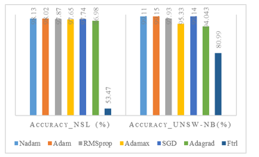
Figure 3: Optimizer Vs. Accuracy

4.2.  Experiment: Learning rate Vs. model performance

The learning rate, a positive scalar multiplied by gradient descent gradient, controls the step size in parameter space. A higher rate facilitates faster convergence but raises the risk of overshooting and oscillation. On the other hand, a lower rate ensures stability but may demand more iterations for convergence.

With optimizers chosen from the preceding Experiment 4.1, the same CNN BLSTM model neural network architecture is used to determine the ideal learning rate to enhance the model performance. The NSL-KDD binary data is preprocessed from the subset of the KDDTrain+ dataset, and the split ratio splits the data for training and testing. The learning rate determines the rate at which new weights are added to neural network models. The other hyperparameters remain constant throughout this experiment while the learning rates are adjusted to optimize the model’s accuracy. Table 6 displays a comparison of learning rate with CNN BLSTM model performance. The model performs best on the UNSW-NB15 binary data and the NSL-KDD binary dataset, achieving a learning rate of 0.01 and 0.0002, respectively. The same learning rate provides different model performances.

Table 6: CNN BLSTM model Learning rate Vs. Performance metrics

Epochs size = 10, Batch = 256, KDD_C2 (Nadam), UNSW-NB15_C2 (adam)
LR	ACC-NSL	F1-NSL	ACC-UN	F1-UN
0.01	97.49	97.67	99.67	99.76
0.001	98.16	98.29	99.54	99.66
0.0001	98.06	98.20	95.81	96.85
0.0002	98.18	98.3	97.9	98.44
0.0003	98.14	98.27	98.44	98.86
0.0004	97.97	98.11	99.13	99.35
0.0005	98.11	98.25	99.09	99.32
LR: Learning rate, ACC: Accuracy in %, F1: F1Score in %, UN: UNSW_NB

4.3.  Experiment: Model dropout rate Vs. model performance

The phrase “dropout rate” in machine learning usually refers to a regularization method that neural networks employ to avoid overfitting. When a model becomes overfit, it can have poor generalization on new, unknown data because it has learned the training set too well, including its noise and outliers. During training, randomly selected neurons (units) in the neural network are “dropped out” or omitted temporarily. This means these neurons do not contribute to the forward or backward pass during a particular iteration of training. The probability of a neuron being dropped out is called the dropout rate. The dropout rate is one hyperparameter that must be determined before training the model.

The CNN BLSTM model was tested and trained for both datasets using a batch size of 256 and 10 epochs. Different dropout rate values were used to evaluate the efficiency of the model. The model performed better than the others, with a 30% dropout rate on the UNSW-NB15 dataset; however, a 60% dropout rate worked better for the NSL-KDD. The hyperparameter values, dropout rates, and corresponding performance metrics are presented in Table 7. The experimental results highlight the varying dropout rates for distinct datasets despite the similarity between the two datasets.

Table 7: Dropout rate Vs. model performance

Epochs size = 10, batch = 256, KDD_C2 (madam), UNSW-NB15_C2 (adam)
DropOut %	ACC-NSL	F1-NSL	ACC-UN	F1-UN
0.1	98.10	98.24	97.44	98.15
0.2	98.02	98.16	98.98	99.25
0.3	98.16	98.29	99.87	99.9
0.4	98.04	98.17	99.27	99.47
0.5	97.93	98.09	99.47	99.61
0.6	98.21	98.33	99.81	99.86
0.7	98.01	98.15	99.58	99.69
0.8	98.04	98.18	98.57	98.94
ACC: Accuracy in %, F1: F1Score in %, NSL: KDD-NSL, UN: UNSW_NB KDDTrain+, UNSW-NB15 training.csv binary with test-train split

      The batch size is a hyperparameter in machine learning that determines how many samples are used in a training iteration. The batch size represents the number of samples used in a single training iteration. Using a smaller batch size incorporates a limited number of data samples and results in a longer training time for the CNN Bi-LSTM model compared to a larger batch size. Throughout experimentation (Experiment A-C), the batch size is altered while maintaining other hyperparameters, such as a fixed number of epochs is 5, the learning rate of the optimizer, and the dropout rate values assigned to the model based on previous findings with the respective datasets.

Table 8: Model performance Vs. batch size

Number of Epochs = 5, KDD_C2 (Nadam), UNSW-NB15_C2(adam)
Batch	ACC-NSL %	F1-NSL %	ACC-UN %	F1-UN %
32	97.89	98.04	99.40	99.55
64	97.95	98.10	99.35	99.52
128	98.06	98.20	99.33	99.50
256	97.64	97.79	96.36	97.26
512	97.92	98.08	96.90	97.70

      The dataset size, the amount of computing power available, and the specifics of the optimization issue can all influence the batch size decision. Experimenting with various batch sizes is a frequent way to determine which is most effective for a certain task.

      The experimental result in Table 8 demonstrates how the neural network’s hyperparameter combinations affect performance. In this experiment, batch sizes of 128 for the binary NSL-KDD datasets and 32 for the binary UNSW-NB15 datasets for epochs 5 demonstrated the best performance of the CNN BLSTM model.

4.4.  Experiment: Epochs Vs. model performance

An “epoch” in machine learning is one whole iteration through the training dataset a model goes through while training. The learning method processes the complete dataset throughout each epoch, modifying the neural network weights and parameters to reduce the error or loss function. A hyperparameter called epoch count determines an algorithm’s running frequency over the full training dataset. The integer between one to infinity can be used as the epoch. Selecting smaller epoch values results in a longer training time for the model and vice versa. Underfitting, the ML model cannot identify the original patterns in the data, which can be caused by using too few epochs. However, an excessive number of epochs might cause overfitting, in which case the model becomes inattentive to new data and underperforms on previously unknown data.

      The CNN BLSTM hybrid model performance for binary KDD-NSL and binary UNSW-NB15 with the different values of epochs are documented in Table 9. The performance increases with large values of epochs but is different for a while. After 75 epochs, the model performance decreases. The amount of data utilized for training and testing, the size of the output class, and other hyperparameter combinations affect the epochs and performance of the machine learning/deep learning models.

Table 9: Epochs Vs. model performance

Batch size = 256, NSL- KDD_C2 (Nadam)
Number of Epochs	Accuracy-NSL %	F1Score-NSL %
2	95.48	95.94
10	98.13	98.26
25	98.21	98.33
50	98.20	98.33
75	98.27	98.39
100	98.26	98.39

      The selection of epoch size to produce a superior performance on an imbalanced dataset is challenging. The binary dataset is more balanced than the multiclass network-based intrusion dataset. The experimental results in Table 9 are not the determining experiment for the number of epochs on multiclass NSL-KDD and UNSW-NB15 datasets. Hence, we experimented with and documented multi-class experimental results to determine the values of epochs where we can produce higher accuracy on the provided dataset. Tables 10 and 11 show the experimental results for multiclass datasets to investigate the values of epochs to make superior detection accuracy. In summary, while epoch size and class size are conceptually different, they can influence each other indirectly, especially when dealing with imbalanced datasets. Selecting the right number of epochs for a given problem is crucial, as is keeping an eye on how class sizes affect model performance.

Table 10: Model performance Vs. Epochs on UNSW-NB15 multiclass data

Batch=512, Optimizer=SGD, Training=UNSW-NB15Train.csv82332 testing data= UNSW-NB15Test.csv175341, Multiclass=10
Epochs	ACC	wt_Prec	wt_F1Score	Prg_exe_time
10	93.10	91.10	91.94	0.64
25	83.09	79.94	79.69	1.17
50	86.4	82.47	83.35	2.24
75	87.1	86.46	85.24	3.12
100	90.04	88.36	88.01	4.24
150	82.23	81.49	80.82	6.36
200	81.13	78.65	78.84	7.95
ACC: Accuracy in %, wt_Prec: weighted Precision in %, wt_F1Score: weighted F1Score in %, Prg_exe_time: Program script run time in hr.

      Program execution time is the sum of the model’s training and testing phases. The program execution time depends on various factors, such as the neural network’s architecture, training and testing data size, class size, and combination of hyperparameters. We documented the performance of the CNN BLSTM hybrid model along with the program execution time. The higher the epochs result, the longer the program execution time. Table 10 and Table 11 show the multi-class NSL-KDD run for almost 8 Hrs. to complete training testing and evaluate the model for 200 epochs. A similar scenario for multiclass UNSW-NB15 dataset. Hence, selecting epoch and batch size is the trade-off with the model training, testing, and evaluation time.  We found in Table 10 and Table 11 the different epoch sizes for NSL-KDD (outperform at epoch size 10) and UNSW-NB15 (outperform at epoch 100) during multi-class model performance.

Table 11: Performance Vs. epochs on NSL-KDD multiclass data

Batch=512, Optimizer= Adam, Data=KDDTrain+_125973, KDDTest+_22544, Multiclass = 5
Epochs	ACC	wt_Prec	wt_F1Score	Prg_exe_time
10	86.21	88.13	83.85	0.45
25	86.64	88.01	84.1	1.08
50	86.64	88.7	84.78	2.15
75	87.11	88.39	84.84	3.31
100	87.63	89.85	86.44	4.53
150	87.22	89.66	85.81	7.03
200	86.84	90.61	86.41	8.76
ACC: Accuracy in %, wt_Prec: weighted Precision in %, wt_F1Score: weighted F1Score in %, Prg_exe_time: Program script run time in hr.

4.5.  Experiment: Imbalance data sampling Vs. performance

This experiment investigates the sampling techniques for imbalanced data to provide a high detection rate.  The researcher employed various techniques, such as a critical selection of ML and DL algorithms, ensemble methods, data sampling, etc., to address the issue of data imbalance because there are fewer attacks than typical traffic data in the provided network intrusion detection dataset.

      Sampling methods generate or delete random data from the dataset based on class data distribution. Random under-sampling and random over-sampling are two techniques used in imbalanced classification problems, where one class (usually the minority traffic class) is significantly under-represented compared to the other class(es). These methods are utilized to tackle class imbalance and enhance the efficacy of machine learning models. Random Under Sampling (RUS) involves randomly removing instances from the majority class until the distribution between the majority and minority classes is more evenly distributed. However, random over-sampling produces an equal distribution by randomly duplicating minority class instances or creating synthetic instances to increase the number of minority class instances.

      Tables 12 and 13 provide the hyperparameter information and performance of this experiment’s CNN BLSTM hybrid model. Table 12 compares the NSL-KDD multiclass dataset’s performance when random over- and under-sampling is applied. After preprocessing multi-class NSL-KDD data, the training and testing datasets merge into a single file. Sampling is implemented on merged data, and a 70:30 split ratio is used to split data into train and test datasets.

Table 12: CNN BLSTM performance Vs. Sampling on NSL-KDD

CNN BILSTM, Epochs= 25, Batch_size= 512, Data = combine (KDDTrain+KDDTest+) (sampling)
Class	Recall_RUS	F1_RUS	Recall_ROS	F1_ROS
DoS	0	0	99.86	99.92
Probe	100	36.69	99.89	99.91
U2R	10	18.18	100	99.73
R2L	0	0	99.45	99.63
Normal	0	0	99.93	99.93
Wt_Average à	22.15	10.07	99.83	99.83
Macro_Avgà	22	10.97	99.83	99.83
Accuracy %	22.15		99.83
[F1:F1Score, RUS: Random Under Sampling, ROS: Random Over Sampling] %

      Similarly, preprocessed training data and testing data files are merged into a single file to implement the sampling method on the UNSW-NB15 multiclass dataset. The sampled data is then split into training and testing datasets using a 70:30 train-test split ratio During Random under-sampling, data instances are randomly deleted from the majority class, resulting in significant information loss. Deleting samples from the majority class results in a smaller sample, unsuitable for the deep learning model and worsens the model performance, which is found in the experiment and documented in Tables 12 and Table 13. Random over-sampling (ROS) helps prevent information loss, as none of the minority class instances are removed. It can be more effective when the amount of data in the minority class is limited.

Table 13: Model performance Vs. sampling on UNSW-NB15

CNN_BLSTM Epochs=25, Batch_size=512, data = combine (UNSW-NB15training-set_175341+UNSW-NB15testing-set_82332) sampling
Class	Recall_RUS	F1_RUS	Recall_ROS	F1_ROS
Analysis	0	0	100	100
Backdoor	0	0	100	100
DoS	0	0	100	99.95
Exploits	100	17.51	99.91	99.95
Fuzzers	0	0	99.98	99.99
Generic	0	0	99.98	99.98
Normal	0	0	100	100
Reconnaissance	0	0	100	100
Shellcode	0	0	100	100
Worms	0	0	100	100
Weighted_Average	9.2	1.61	99.99	99.99
Macro Average	10	1.75	99.99	99.99
Accuracy (%)	9.20		99.99
[F1:F1Score, RUS: Random Under Sampling, ROS: Random Over Sampling] %

      This method generates random data based on the data distribution in the dataset. The huge amount of data is always suitable for deep learning models. Regarding detection accuracy, our suggested CNN BLSTM hybrid model performs better than the random over-sampling technique, offering over 99%. Tables 12, 13, and Figure 4 above detailed the CNN BLSTM hybrid model’s performance for the UNSW-NB15 imbalance dataset and the multiclass NSL-KDD.

5. Conclusion

The previous research from the literature reviews shows that while the detection accuracy for rarely occurring attack classes (U2R, R2L) is low, the average model accuracy for normal traffic in the UNSW-NB15 and NSL-KDD is roughly 99%. Regardless of the type of attack, each poses a threat to network machines equally. To provide a comparative analysis, we juxtapose our results with existing findings of 91.12% [20] and 90.83% [5] detection accuracy for NSL-KDD binary, and 99.70% [18], 82.08% [14], 82.08% for UNSW-NB15 binary datasets. Our experiments enhance accuracy to 98.27% on NSL-KDD and 99.87% on UNSW-NB15 binary datasets by carefully selecting hyperparameters and conducting various experiments. We explored the CNN BLSTM hybrid model’s hyperparameters (dropout. epochs, batch size, learning rate, and optimizer) to maximize detection accuracy for the binary NSL-KDD and UNSW-NB15.

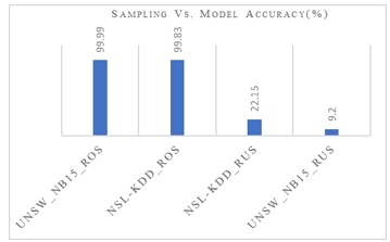
Figure 4: Sampling Vs. multiclass model accuracy (%)

The model performance depends on the combination of hyperparameters, the size of the dataset used to train/test the model, and the selection of the machine learning/ deep learning model. Our research provides information about the data size used during the experiments and the choice of hyperparameters. The suggested model uses random over-sampling techniques on a single set of data to provide 99.99% and 99.83% model accuracy for the multiclass UNSW-NB15 and NSL-KDD datasets, respectively (train and test data merge into a single file before sampling).

      Selecting random over-sampling or under-sampling relies on the particulars of the dataset and the issue at hand. To achieve a balance, combining the two methods, a practice known as hybrid sampling may occasionally be necessary. It’s crucial to remember that there are more sophisticated methods for dealing with class imbalance, such as SMOTE (Synthetic Minority Over-sampling Technique), which creates synthetic instances for the minority class instead of merely copying real instances. Thoroughly examining those approaches in various network intrusion detection multiclass datasets extends this research effort. The proper use of hyperparameters of neural networks, size of dataset used to train the model, and sampling methods for CNN BLSTM network anomaly model provide the highest detection accuracy for imbalance network data.

Conflict of Interest

The authors declare no conflict of interest.

Acknowledgment

The National Science Foundation (NSF) and Scholarship for Service CyberCorps (SFS CyberCorps) programs support this research study. The award information of NSF and CyberCorps are #1910868 and #2219611, respectively. This cannot be completed without the continuous support of advisors and the Electrical and Computer Engineering Departments of Prairie View A&M University

1. T. Acharya, A. Annamalai, M.F. Chouikha, “Efficacy of CNN-Bidirectional LSTM Hybrid Model for Network-Based Anomaly Detection,” in 13th IEEE Symposium on Computer Applications and Industrial Electronics, ISCAIE 2023, Institute of Electrical and Electronics Engineers Inc.: 348–353, 2023, doi:10.1109/ISCAIE57739.2023.10165088.
2. N. Moustafa, J. Hu, J. Slay, “A holistic review of Network Anomaly Detection Systems: A comprehensive survey,” Journal of Network and Computer Applications, 128, 33–55, 2019, doi:10.1016/j.jnca.2018.12.006.
3. H. Liu, B. Lang, M. Liu, H. Yan, “CNN and RNN based payload classification methods for attack detection,” Knowledge-Based Systems, 163, 332–341, 2019, doi:10.1016/j.knosys.2018.08.036.
4. B. Cao, C. Li, Y. Song, Y. Qin, C. Chen, “Network Intrusion Detection Model Based on CNN and GRU,” Applied Sciences (Switzerland), 12(9), 2022, doi:10.3390/app12094184.
5. Y. Fu, Y. Du, Z. Cao, Q. Li, W. Xiang, “A Deep Learning Model for Network Intrusion Detection with Imbalanced Data,” Electronics (Switzerland), 11(6), 2022, doi:10.3390/electronics11060898.
6. X. Ji, H. Zhang, X. Ma, “A Novel Method of Intrusion Detection Based on Federated Transfer Learning and Convolutional Neural Network,” in IEEE Joint International Information Technology and Artificial Intelligence Conference (ITAIC), Institute of Electrical and Electronics Engineers Inc.: 338–343, 2022, doi:10.1109/ITAIC54216.2022.9836871.
7. T. Acharya, I. Khatri, A. Annamalai, M.F. Chouikha, “Efficacy of Heterogeneous Ensemble Assisted Machine Learning Model for Binary and Multi-Class Network Intrusion Detection,” in 2021 IEEE International Conference on Automatic Control and Intelligent Systems, I2CACIS 2021 – Proceedings, Institute of Electrical and Electronics Engineers Inc.: 408–413, 2021, doi:10.1109/I2CACIS52118.2021.9495864.
8. T. Acharya, I. Khatri, A. Annamalai, M.F. Chouikha, “Efficacy of Machine Learning-Based Classifiers for Binary and Multi-Class Network Intrusion Detection,” in 2021 IEEE International Conference on Automatic Control and Intelligent Systems, I2CACIS 2021 – Proceedings, Institute of Electrical and Electronics Engineers Inc.: 402–407, 2021, doi:10.1109/I2CACIS52118.2021.9495877.
9. M. Xiong, H. Ma, Z. Fang, D. Wang, Q. Wang, X. Wang, “Bi-LSTM: Finding Network Anomaly Based on Feature Grouping Clustering,” in ACM International Conference Proceeding Series, Association for Computing Machinery: 88–94, 2020, doi:10.1145/3426826.3426843.
10. S.N. Pakanzad, H. Monkaresi, “Providing a hybrid approach for detecting malicious traffic on the computer networks using convolutional neural networks,” in 2020 28th Iranian Conference on Electrical Engineering, ICEE 2020, Institute of Electrical and Electronics Engineers Inc., 2020, doi:10.1109/ICEE50131.2020.9260686.
11. R. Yao, N. Wang, Z. Liu, P. Chen, X. Sheng, “Intrusion detection system in the advanced metering infrastructure: A cross-layer feature-fusion CNN-LSTM-based approach,” Sensors (Switzerland), 21(2), 1–17, 2021, doi:10.3390/s21020626.
12. P. Sun, P. Liu, Q. Li, C. Liu, X. Lu, R. Hao, J. Chen, “DL-IDS: Extracting features using CNN-LSTM hybrid network for intrusion detection system,” Security and Communication Networks, 2020, 2020, doi:10.1155/2020/8890306.
13. L. Zhang, J. Huang, Y. Zhang, G. Zhang, “Intrusion Detection Model of CNN-BiLSTM Algorithm Based on Mean Control,” in Proceedings of the IEEE International Conference on Software Engineering and Service Sciences, ICSESS, IEEE Computer Society: 22–27, 2020, doi:10.1109/ICSESS49938.2020.9237656.
14. J. Sinha, M. Manollas, “Efficient Deep CNN-BiLSTM Model for Network Intrusion Detection,” in ACM International Conference Proceeding Series, Association for Computing Machinery: 223–231, 2020, doi:10.1145/3430199.3430224.
15. A. Li, S. Yi, “Intelligent Intrusion Detection Method of Industrial Internet of Things Based on CNN-BiLSTM,” Security and Communication Networks, 2022, 2022, doi:10.1155/2022/5448647.
16. J. Gao, “Network Intrusion Detection Method Combining CNN and BiLSTM in Cloud Computing Environment,” Computational Intelligence and Neuroscience, 2022, 2022, doi:10.1155/2022/7272479.
17. T. Acharya, A. Annamalai, M.F. Chouikha, “Efficacy of Bidirectional LSTM Model for Network-Based Anomaly Detection,” in 13th IEEE Symposium on Computer Applications and Industrial Electronics, ISCAIE 2023, Institute of Electrical and Electronics Engineers Inc.: 336–341, 2023, doi:10.1109/ISCAIE57739.2023.10165336.
18. P. TS, P. Shrinivasacharya, “Evaluating neural networks using Bi-Directional LSTM for network IDS (intrusion detection systems) in cyber security,” Global Transitions Proceedings, 2(2), 448–454, 2021, doi:10.1016/j.gltp.2021.08.017.
19. Y. Imrana, Y. Xiang, L. Ali, Z. Abdul-Rauf, “A bidirectional LSTM deep learning approach for intrusion detection,” Expert Systems with Applications, 185, 2021, doi:10.1016/j.eswa.2021.115524.
20. W. Xu, J. Jang-Jaccard, T. Liu, F. Sabrina, J. Kwak, “Improved Bidirectional GAN-Based Approach for Network Intrusion Detection Using One-Class Classifier,” Computers, 11(6), 2022, doi:10.3390/computers11060085.
21. T. Acharya, A. Annamalai, M.F. Chouikha, “Optimizing the Performance of Network Anomaly Detection Using Bidirectional Long Short-Term Memory (Bi-LSTM) and Over-sampling for Imbalance Network Traffic Data,” Advances in Science, Technology and Engineering Systems Journal, 8(6), 144–154, 2023, doi:10.25046/aj080614.
22. M. and B.E. and L.W. and G.A.A. Tavallaee, “A detailed analysis of the KDD CUP 99 data set,” in 2009 IEEE Symposium on Computational Intelligence for Security and Defense Applications, IEEE, 2009, doi:{10.1109/CISDA.2009.5356528}.
23. L. Dhanabal, S.P. Shantharajah, “A Study on NSL-KDD Dataset for Intrusion Detection System Based on Classification Algorithms,” International Journal of Advanced Research in Computer and Communication Engineering, 4, 2015, doi:10.17148/IJARCCE.2015.4696.
24. N. Moustafa and J. Slay, “UNSW-NB15: a comprehensive data set for network intrusion detection systems (UNSW-NB15 network data set),” 2015 Military Communications and Information Systems Conference (MilCIS), Canberra, ACT, Australia, 2015, pp. 1-6, doi: 10.1109/MilCIS.2015.7348942.