1. Introduction

In the year 2020, liver cancer affected more than 900,000 individuals globally, leading to over 830,000 deaths. It ranks sixth among the top ten cancers worldwide and is the primary cancer in the United States [2]. Accordingly, it is crucial to conduct research on the expression of symptoms in adult liver cancer to facilitate clinical intervention. Previous research on symptoms for Liver Carcinoma and Cancer have provided valuable insights, with physical searches of article references yielding additional findings [3]. Logic-based approach such as supervised models, including linear regression, decision trees, association learning algorithms such as Random Forest and Generalized Boosting Machines, and Support Vector Machines (SVM), are commonly employed in this field. SVMs use a polynomial kernel function and a non-probabilistic approach [4]. Decision trees are an example of a prognostic model that maps entity attributes and values. Each intersection in the tree represents an entity, each bifurcation path represents a potential attribute value, and each leaf intersection correlate with the entity value appear for by the direction from the root junction to the leaf junction. Although decision trees have a single output, multiple trees can be utilized to handle various outputs. This technology is commonly utilized in data mining [5].

In the field of liver cancer, decision tree models can be employed to categorize patients based on their symptoms and forecast the possibility of developing liver cancer or their prognosis post-diagnosis. Decision tree models can also be combined with other machine learning algorithms to enhance precision and credibility [6].

APRIORI algorithms like Random Forest and Generalized Boosting Machines are frequently utilized supervised models for liver cancer prediction [7]. Random Forest is a decision tree-based association learning technique that establish multiple decision trees and returns the approach of the class predictions from individual trees [8]. On the other hand, Generalized Boosting Machines is an iterative algorithm that constructs a strong model by combining several weak models, with each weak model aiming to rectify the errors of the previous one [9].

2. Previous work

This section presents an overview of the main machine learning techniques utilized in the analysis of the Hepatitis dataset obtained from CARNEGIE-MELLON University in 1988, as part of the Statlog project. The outcomes of the analysis, performed with and without 10-fold cross-validation, are combined into a consolidated form for the purpose of comparison and assessment.

Table. 1 The analysis outcome of hepatitis data provided major from Statlog project

This study presents a comprehensive comparative analysis of machine learning methods conducted by various authors, including M. Ramassamy, S. Selvaraj, M. Mayilvaganan, and Bascil & Temurtas. Notable methodologies include PCA+AIRS with 94.12% accuracy rate by Kemal Polat and Salih Güneş [10]. Other accuracy rates including 21-NN (stand. Manhattan) with 90.3%, FSM with 90% and 14-NN with 89% by Statlog project, and LDA with 86.4%, CART (decision tree) with 82.7%, and MLP+backprop by Weiss & K with 82.1% [11]. Duch & Grudzinski applied Weighted 9-NN with 92.9%±?, 18-NN (stand. Manhattan) with 90.2±0.7, and 15-NN (stand. Euclidean) with 89.0±0.5% [12], while Rafa Adamczak employed FSM with rotations with 89.7±? and FSM without rotations with 88.5% [13]. Stern & Dobnikar utilized a diverse set of methods, including LDA (linear discriminant analysis) with 86.4% accuracy rate, Naive Bayes and Semi-NB with 86.3%, 1-NN (stand. added by WD) with 85.3%±5.4, ASR with 85%, Fisher discriminant analysis with 84.5%, LVQ with 83.2%, CART (decision tree) with 82.7%, MLP with BP with 82.1%, ASI with 82%, and LFC with 81.9% [14]. Norbert Jankowski implemented IncNet with 86% accuracy rate [15]. These findings collectively contribute valuable insights into the efficacy of distinct machine learning approaches for addressing statistical learning challenges. Within the framework of the Statlog project, machine learning methodologies have demonstrated substantial efficacy in analyzing Hepatitis data, with the PCA+AIRS model outperforming others, achieving an accuracy rate of 94.12%.

Data Mining is getting increasingly important for discovering association patterns for health service innovation and Customer Relationship Management (CRM) etc. Yet, there are deficits of existing data mining techniques. First of all, most of them perform a plain mining based on a predefined schemata through the data warehouse; however, a re-scan must be done whenever new attributes appear. Second, an association rule may be true on a certain granularity but fail on a smaller one and vise verse. Last but not least, they are usually designed to find either frequent or infrequent rules. In this paper, we are going to invent more efficient and accurate approach with novel data structure and multi-dimensional mining algorithm to explore association patterns on different granularities [16] [17].

The paper presents at first the categories of innovative healthcare services as well as the way to find new service patterns. Then, we propose a data mining approach based on Apriori Algorithm for managing such new healthcare services, including a novel data structure and an effective algorithm for multi-dimensional mining association rules on various granularities. It is proved to be very useful for discovering new service patterns, even in-frequent by considering a dimension in a flat level. The advantages of this approach over existing approaches include (1) more comprehensive and easy-to-use (2) more efficient with limited scans (3) more effective with finding rules hold in different granularity levels, e.g. Age={(1-10), (10-20)….} (4) capable of finding frequent patterns and infrequent patterns, for instant we use the algorithm in finding the blood platelet frequently used for the female with age over 60, while the blood platelet infrequently for all the patients. With this method, users can choose the full match and the relaxed match (5) low information loss rate (6) capable of incremental Mining.

3. Data pre-processing

3.1.  Field attributes

The majority of the primary dataset comprises symptom information, and therefore, the values in the range are predominantly binary (i.e., negative or positive). The dataset comprises 6 numeric and 14 categorical attributes, amongst the Class attribute is ranked in accordance with the form presented in reference [18].

Table 2: Hepatitis symptoms selected by Carnegie Mellon University

3.2 Data pre-processing

1. Attribute analysis

Upon importing the raw data, an intrinsic attribute analysis was conducted utilizing the WEKA software to scrutinize the data pertaining to each attribute. [19].

1. Data preprocessing

Prior to data analysis, data preparation is a necessary step which involves data preprocessing and data reduction. The primary goal of data preprocessing is to address impure, incomplete or inconsistent data within the original dataset. Meanwhile, data reduction aims to decrease the volume or dimensionality of the initial data, for the purpose of alleviate the burden of data exploration. The significance of data preparation is demonstrated in the following scenarios: Firstly, the data may contain noise, such as errors or outliers resulting from issues with data collection equipment, human or computer errors during data recording or transmission, etc. Secondly, the data may be incomplete, with some attribute values missing due to reasons such as unnecessary data being excluded during recording or inconsistent records being deleted. Finally, inconsistency may also arise when the same data has multiple conflicting conditions, for instance, when the data is integrated from various sources with different naming conventions.

Data conversion is a critical step in data preprocessing that seeks to transform missing or inaccurate data into a compatible format for the exploration process. This research utilized four distinct preprocessing techniques, namely data discretization, data extreme value handling, data standardization, and data normalization, to enhance the quality of the data.

• Discretization of data

In order to absolve impoverished classification quality, continuous data is discretized to reduce the numerical allocation of the information.

• Data standardization

To normalize attribute data values and bring them into a minor and consistent range with other attribute data, various techniques can be used, such as Min-Max standardization, z-score standardization, and decimal standardization. The diagram below illustrates the attribute analysis of the initial data after standardization.

• Data normalization

Normalization is a data processing technique used to adjust the data values to a common scale or range. This is done to make the data comparable and reduce the impact of different measurement units or scales on data analysis. For instance, when comparing the annual income of customers in Taiwan and the Philippines, it is not appropriate to directly compare the income levels in Taiwan dollars, as the average income in Taiwan is much higher than that in the Philippines. Therefore, normalization is used to redistribute the data into a small and specific range, which allows for objective and meaningful comparisons.

The aforementioned data processing was carried out utilizing the configurations provided by WEKA.

1. Data reduction

Data reduction is a crucial technique that involves reducing the size or dimensions of data without significantly impacting the exploration outcomes. The main object of data reduction is to ease the burden of data exploration, reduce computation time, improve prediction accuracy, and enhance exploration outcomes’ quality by removing irrelevant or unnecessary data. Information Gain, Gini Index, and χ2 independence test are common characteristic selection criteria used in data reduction. In this research, Information Gain is used as the attribute selection standard to remove attributes with the lowest direction gain value to prepare for the J48 data classification method in WEKA (Waikato Environment for Knowledge Analysis). Information Gain measures the difference between the information quantity before and after a test, represented by the entropy value of the sub-decision tree (Entropy), which is the entropy value of the set produced by a junction with a particular characteristic as the conclusion number. However, Information Gain-based attribute selection may be biased towards attributes with more attributes, resulting in biased decisions. To address this issue, the Gain Ratio method normalizes the Information Gain by dividing it by the number of possible attribute values, preventing bias towards attributes with more qualitative attributes.

By using the conducting analysis, it was observed that attribute 9 and attribute 10 exhibit the lowest information gain and gain ratio. Consequently, these two attributes are eliminated to diminish the data dimensionality. Subsequent to data reduction, the data preprocessing procedures, comprising data discretization, standardization, and regularization, are implemented anew to finalize the data preprocessing stage.

4. Data analysis:

4.1. Classification

4.1.1. Decision tree:

In the realm of machine learning, a decision tree is an example used to predict a mapping connection between characteristic and their respective values. Each junction in the tree denotes a task, and every branching path indicates a feasible characteristic value. The terminal nodes correspond to the values of the objects represented by the paths from the root junction to the terminal junctions. A decision tree has a solitary output, and to address multiple outputs, distinct decision trees can be constructed. Decision trees are a frequently employed approach in data mining for the purpose of analyzing and predicting data.

• Categorical decision tree: target variable is categorical

Categorical decision tree examination is a machine learning tactic used when the target variable is categorical in nature, such as predicting the species of a plant or the likelihood of a customer to purchase a product. This approach is implemented using various algorithms, including ID3, C4.5 (J48), and C5.0.

• Regression decision tree: target variable is continuous

Regression decision tree analysis involves the use of decision trees to predict continuous numerical values, such as the temperature or stock price. It is a widely used technique in data analysis and machine learning. Several algorithms can be used to implement regression decision tree analysis, such as CART, CHAID (Chi-Square Test), MP (multivariate polynomial) and C4.5 (Gain Ratio).

1. J48 Algorithm

J48 is a decision tree algorithm that is based on the C4.5 implementation. The creator of C4.5 later upgraded the algorithm to C4.8, which was then implemented in Java by the creators of Weka and named J4.8. The ID3 algorithm must be introduced first because the C4.5 algorithm is an improved version of ID3.

During the construction of the decision tree, the ID3 algorithm uses Information Gain as the criterion to select the attribute with the highest information gain value as the classification attribute. This algorithm is based on the principle of Occam’s razor, which states that the smaller the decision tree, the preferable the exhibition. However, the ID3 algorithm is a heuristic algorithm and may not always produce the smallest tree structure. Moreover, one of the issues with ID3 is its bias towards attributes with multiple values. For example, if there is a distinctive recognition characteristic such as an ID, ID3 may choose it as the splitting characteristic. Although this creates a sufficiently clean section, it is nearly futile for classification purposes. To address this problem, the C4.5 algorithm, which is the successor of ID3, employs the gain ratio information obtain extension to reduce this bias.

4. C4.5:

C4.5 is a set of algorithms frequently utilized in machine learning and data mining for classification tasks. Specifically, its purpose is to perform supervised learning, where a dataset contains tuples characterized by attribute values and each tuple belongs to one of several exclusive categories. The aim of C4.5 is to construct a mapping function from the attribute values to categories that can be used to classify new instances with unknown categories.

4. Ross Quinlan proposed C4.5 as an extension of the ID3 algorithm, which is used to construct decision trees. A decision tree is a tree-like structure similar to a flowchart, where each internal node presents an attribute exam, each branch presents an exam outcome, and each leaf node reserves a class label. After the decision tree is constructed, an unclassified tuple can be traversed from the root node to a leaf node, which stores the predicted class label for the tuple. Decision trees are advantageous because they do not postulate any prior estate expertise or guideline settings and are appropriate for investigative comprehension discovery.

C4.5 overcomes the problems of ID3 by adopting the gain ratio of attributes, which normalizes the information gain by computing the break knowledge value of the virtue. In the C4.5 algorithm, the break apart virtue selection process does not solely rely on the virtue with the supreme gain ratio. Instead, it searches for attributes that have a direction obtain higher than the standard level among the candidate separation virtue, and then choice the virtue with the supreme gain ratio. This is because gain ratio tends to favor attributes with smaller values compared to information gain.

C4.5 has several improvements over ID3. Firstly, it can handle continuous attributes. Secondly, it uses gain ratio to overcome ID3’s bias towards attributes with many distinct values but little significance. This is because the guidance obtain measure used by ID3 inclines to select virtue with many distinct values, which can lead to the creation of suboptimal decision trees. For example, if the algorithm divides the data based on a unique attribute like student ID, it would generate numerous branches, each with only one or a few instances, resulting in a high information gain value but a meaningless split.

Table 3. J48 Results Comparison Table

Attribute	Accuracy Rate
Whole samples	90.3226%
Cross Validation	84.5161%
66% Training data	81.1321%

4.1.2. The principle of CART algorithm

As previously stated, the CART algorithm comprises two stages, and in the first stage, a binary tree is constructed recursively. The question then arises: how is the data divided?

In the field of machine learning and data mining, the CART algorithm is often employed for classification tasks, where each data point is assigned to one of several exclusive categories based on a selected attribute. The algorithm divides the multidimensional space recursively into non-overlapping rectangular regions through a process that involves selecting independent variables and partitioning the space based on the values of the selected variable. The procedure is duplicated circularly on each of the resulting areas until the entire space is covered by non-overlapping regions.

The standard for dividing the space is an important consideration in the CART algorithm. For variable attributes, the dividing point is typically determined as the middle between a pair of endless variable virtue values. The amount of adulteration that can be reduced by dividing on each attribute is then calculated and used to sort the attributes. The decrease of adulteration is explicit as the aggregate of the amount of adulteration before separates minus the amount of adulteration at each node after division. The Gini index is routinely accustomed to as a method for measuring adulteration. Gini impurity measures the probability that a given node represents a certain class, and it is minimized when all samples in the node belong to the same class.

The core concept of the CART algorithm is to recursively classify data based on a minimum distance-based Niki index estimation function. One of the main benefits of the algorithm is its simple and easy-to-understand rule extraction process. Moreover, the CART algorithm is robust against issues such as missing values and a large number of variables, making it a widely used and effective tool in machine learning and data mining.

Algorithm limitations: attribute selection is restricted to generating only two child nodes; error rate may increase rapidly with a large number of categories.

Application domains: identification of information distortion, identification of potential customers in the telecommunications industry, prediction of loan risks, and others.

Table 4. CART Results Comparison Table

Attribute	Accuracy Rate
All samples	90.3226%
Cross-Validation	84.5161%
66% of Samples	81.1321%

1. J48 VS CART

The fundamental distinction between CART and J48 algorithms lies in the criterion used to split the nodes. CART adopts the GINI index to measure the purity of data partitions or training datasets when choosing a splitting attribute. The GINI index quantifies the purity of a sample based on the likelihood of it belonging to a specific category. Consequently, the attribute that results in the minimum GINI index is selected for division.

Table 5. Classification results analysis

Algorithm	Pre-process	Test mode	Accuracy Rate
J48	Normalization	Whole sample	87.0968%
J48	Normalization	Cross Validation	85.1613%
J48	Normalization	66% Training data	88.6792%
CART	Normalization	Whole sample	90.3226%
CART	Normalization	Cross Validation	94.5161%
CART	Normalization	66% Training Data	81.1321%

4.2. Association Law (APRIORI)

Within a vast bibliography, interrelationships among specific purposes exist, commonly referred to as Market Basket Analysis, which originated from analyzing the extent of conjunction of sizeable itemsets in merchandise case data. This analysis utilizes the law of association, frequently used in the study of shopping baskets, to examine the correlation between purchased products in customer acquire data recorded by the POS system. An exemplary illustration of the law of association is the well-known paradigm of the correlation between beer and diapers.

Association rules can be conveyed in the form of X => Y [Support, Confidence], where T={t1, t2, …, tm} represents the set of all items, X⊂T, Y⊂T, and X∩Y=Φ. Here, X and Y denote unique data item sets in the transaction set T, indicating that if X emerge, Y may also emerge concomitantly. The assist of an association rule X Y in T, performed by support (X Y) = P(X Y) = s, is the ratio of agreement including X∩Y to all agreement in T. The accreditation of an association rule X Y in T, served by confidence (X Y) = P (Y|X) = c, is the ratio of agreements including X∩Y to agreements including X in T. The values of support and confidence range between 0 and 1.

An item set (itemset) refers to a collection of distinct items, such as {A, B, C} in a record, which can produce the item group {A}, {B}, {C}, {A, B}, {B, C}, {A, C}, {A, B, C}. If there are n items in the item set, the item group comprises 2n-1 items. Therefore, when managing a large number of items, the item group can be extensive.

The support (Support) of an item set in the database is the frequency of the item set in the database, typically denoted by Support (X), where X is itemset. For instance, if a database has 100 transaction records, and 40 of them indicate the purchase of milk, then the support of this item set is 40/100=40%. The higher the support, the more crucial the item set is for further exploration.

Confidence (Confidence) signifies the level of trust between two itemsets and is represented by the conditional probability that Y will appear under the probability of X appearing, usually expressed as Support (X∩Y) /Support (X), where X and Y are itemsets.

In the realm of data mining, a robust association rule is characterized by X => Y, a rule that can be established in the transaction set T if it satisfies two conditions: support (A => B) >= min_sup and confidence (A => B) >= min_conf, where min_sup and min_conf indicate the minimum thresholds for support and confidence, respectively. When both of these criteria are met, the rule X => Y is deemed a robust association rule within the transaction set T.

In evaluating association rules, two critical criteria must be met:

The rule should identify unanticipated and unintended associations.

The rule should be capable of making an impact.

One well-known algorithm for generating association rules is Apriori. It employs a bottom-up, iterative approach to identify high-frequency item sets by breading and examination applicant item sets. From these high-frequency item sets, the algorithm identifies useful association rules.

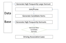
Figure 1: The Apriori algorithm

The Apriori algorithm involves two main steps:

Discovering Large itemsets from the transaction items in the database

The goal is to identify frequent Large itemsets, which requires repeated searches of the database. As Large itemsets have the property that all of their subsets are also frequent, the algorithm generates new sub-itemsets using join and prune operations.

Generating association rules based on the discovered Large itemsets

The Large itemsets obtained in step one are used to derive meaningful association rules. A rule is considered meaningful only if its confidence exceeds the minimum confidence threshold (Min Confidence).

Apriori algorithm process:

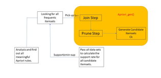
Figure 2: The Apriori process diagram

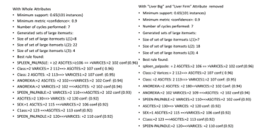
Figure 3. The Apriori result before and after “Liver big” and “Liver Firm” attribute removed.

In the APRIORI algorithm, the first pass through the database is employed to determine the Large 1-itemsets.

For subsequent passes, the algorithm is composed of two stages:

– In the first stage, the Apriori-gen function is utilized to generate new candidate itemsets Ck from the previously discovered Large itemsets Lk-1.

– In the second stage, the database is examined to calculate the Support value of the candidate itemsets in Ck.

The following is the result of the APRIORI algorithm based on our data, before removing “Liver Big” and “Liver Firm” in the APRIORI attribute.

Based on the two datasets provided and the outcomes of the association analysis, it is discernible that a substantive correlation between the “Liver Big” and “Liver Firm” attributes and other pertinent attributes appears to be lacking. The findings are expounded as follows:

In the initial dataset, encompassing both the “Liver Big” and “Liver Firm” attributes, the derived association analysis results are expounded as follows:

The cardinality of the generated large itemsets: L(1)=8, L(2)=22, L(3)=4

Optimal rules identified: Diverse rules, exemplified by instances such as spleen_palpable≥2, Ascites≥106 → Varices=2 conf:(0.96), and comparable formulations.

Conversely, upon the exclusion of the “Liver Big” and “Liver Firm” attributes from the dataset, the ensuing association analysis outcomes are delineated as follows:

The cardinality of the generated large itemsets: L(1)=7, L(2)=18, L(3)=4

Optimal rules identified: Analogous to those observed in the primary dataset, including instances like spleen_palpable=2, Ascites=2 → Varices=2 conf:(0.96), alongside other commensurate rules.

In light of these results, the following rationales can be adduced:

Scarcity of Substantive Rules: In both datasets, conspicuous absence of significant rules directly associating the “Liver Big” and “Liver Firm” attributes with other attributes is noticeable. This indicates a limited propensity for these two attributes to interact significantly with the remaining attributes in the datasets.

Attribute Sparse Occurrence: The rare occurrence of instances wherein the “Liver Big” and “Liver Firm” attributes co-occur with other attributes might be attributed to data scarcity. This scarcity may engender challenges in discerning robust associations between these attributes.

Threshold Specification: The stipulated thresholds for minimum support and confidence, set at 0.65 and 0.9 respectively, might inadvertently sift out associations characterized by lower frequencies and confidence levels. Given the presumed low-level associations of “Liver Big” and “Liver Firm” attributes, adherence to the specified thresholds could preclude their inclusion in the derived association rules.

Data Profile Dynamics: The outcomes are also liable to be influenced by data profile intricacies and distribution patterns. In instances where the “Liver Big” and “Liver Firm” attributes do not manifest as prominent co-occurring features within the dataset, the association analysis might struggle to identify substantial relationships.

In summation, predicated on the proffered datasets and the contextual framework of the association analysis, the dearth of observable significant associations between the “Liver Big” and “Liver Firm” attributes and other pertinent attributes is discernible. This, however, does not conclusively imply a universal lack of connection; rather, it underscores the paucity of apparent associations within the existing conditions and dataset parameters.

5. Discussion and future study

This investigation is fundamentally grounded in the amelioration of machine learning techniques, as opposed to adopting traditional statistical methods. Additionally, it has been observed that mixed methods generally yield higher accuracy levels, thereby substantiating the selection of J48 and the Gini index-based CART algorithm as apt methodologies for this particular study.

It is imperative to acknowledge that both machine learning and AI are continuously evolving fields, and with access to an augmented sample size and the elucidation of additional attributes, there is a potential for even more exemplary performance and a more meticulous analysis.

The Apriori analysis conducted revealed a low correlation between the attributes “Liver Big” and “Liver Firm,” indicating that their removal does not impact the final results significantly. For analyzing relationships such as the variations in age groups, we recommend employing our Multi-dimensional Multi-granularities Data Mining based on the Apriori Algorithm. This approach enables the segmentation of patient ages into various granularities, specifically {(10-20), (20-30), …, (70-80)}. Subsequently, we can mine for association patterns within these defined segments, ensuring that phenomena pertinent to children do not get erroneously associated with adults. However, upon constructing data cubes for age ranges (10-20), (60-70), and (70-80), we may uncover associations within these specific segment combinations or granularities.

6. Conclusion

The consolidation of machine learning with the therapeutic realm presents numerous advantages, such as an improved understanding of disease characteristics and the potential to aid healthcare providers in developing more efficient treatment strategies for patients. Machine learning finds application in diverse areas within the medical sector, not just limited to the employment of qualitative and quantitative material categorization to draw inferences, and association rules to establish links between manifestation. For example, in the domain of oncology, machine learning is utilized in supervised therapeutic photo and quantitative data-based congregate to determine if a tumor is hostile. Furthermore, deep learning and computer vision technologies aid in detecting brain tumors. These advancements are indicative of the maturing machine learning applications in medical treatment. With easily accessible tools, physicians and researchers can obtain precise results and prescribe appropriate medication for symptom management, while the principle population can adopt this knowledge to prevent and improve recognize diseases. The medical field anticipates the emergence of additional machine learning and data mining utilization in the future, extending beyond the treatment of hepatitis.

1. J. K. Chiang and R. Chi, “Comparison of Decision Tree J48 and CART in Liver Cancer Symptom with CARNEGIE-MELLON UNIVERSITY Data,” 2022 IEEE 4th Eurasia Conference on Biomedical Engineering, Healthcare and Sustainability (ECBIOS), Tainan, Taiwan, 28-31, 2022, doi: 10.1109/ECBIOS54627.2022.9945039.
2. Liver cancer deaths in 2020 approaching incidence, https://www.cn- healthcare.com/articlewm/20210115/content-1180778.html.
3. M. E. Cooley, “Symptoms in adults with lung cancer: A systematic research review,” Jounal of Pain and Symptom Management, 19(2), February, 2000.
4. C. M. Lynch, “Prediction of lung cancer patient survival via supervised machine learning MARK classification techniques,” International Journal of Medical Informatics 108, 1-8, 2017.
5. Z. Mahmoodabai, S. S. Tabrizi, “A new ICA-Based algorithm for diagnosis of coronary artery disease,” Intelligent Computing, Communication and Devices, 2, 415-427, 2014.
6. Datasets used for classification comparison of results. https://www.is.umk.pl/~duch/projects/projects/datasets.html#Hepatitis
7. M. Hegland, The APRIORI Algorithm—A Tutorial, https://www.worldscientific.com/doi/abs/10.1142/9789812709066_0006
8. D. Michie, D.J. Spiegelhalter, C.C. Taylor, “Machine Learning, Neural and Statistical Classification,” Ellis Horwood Series in Artificial Intelligence: New York, NY, USA, 13, 1994.
9. S. Touzani, J. Granderson, S. Fernandes, “Gradient boosting machine for modeling the energy consumption of commercial buildings,” Energy and Buildings, 158(1533-1543), 2018, doi: 10.1016/j.enbuild.2017.11.039
10. K. Polat, S. Güneş, “Hybrid prediction model with missing value imputation for medical data, Expert Systems with Applications,” 42(13), 5621-5631, 2015
11. S.M. Weiss, I. Kapouleas, “An empirical comparison of pattern recognition, neural nets and machine learning classification methods,” Department of Computer Science, Rutgers University, New Brunswick, NJ 08903, 1989
12. W. Duch, K. Grudzi´nski, “Weighting and selection of features,” Intelligent Information Systems VIII, Proceedings of the Workshop held in Ustro´n, Poland, 1999
13. N Jankowski, A Naud, R Adamczak, “Feature Space Mapping: a neurofuzzy network for system identification,”, Department of Computer Methods, Nicholas Copernicus University, Poland, 1995
14. B. Stern and A. Dobnikar, “Neural networks in medical diagnosis: Comparison with other methods,” Proceedings of the International Conference EANN ’96, 427-430, 1996.
15. Norbert Jankowski, “Approximation and Classification in Medicine with IncNet Neural Networks,” Department of Computer Methods Nicholas Copernicus University ul. Grudziądzka 5, 87-100, Toruń, Poland, 1999
16. J. K. Chiang, C. C. Chu, “Multi-dimensional multi-granularities data mining for discovering innovative healthcare services,” Journal of Biomedical Engineering and Medical Imaging, 1(3), 214, DOI: 10.14738/jbemi.13.243
17. J. K. Chiang, C. C. Chu, “Multidimensional multi-granularities data mining for discover association rule,” Transactions on Machine Learning and Artificial Intelligence, 2(3), 2014.
18. Hepatitis Data Set. https://archive.ics.uci.edu/ml/datasets/Hepatitis
19. Weka website. https://www.cs.waikato.ac.nz/~ml/weka/

(Click Here)