1. Introduction

Decision Trees (DTs) are an important type of algorithm for predictive modeling machine learning. It’s often used to plan and plot business and operational decisions as a visual flowchart. The approach sees a branching of decisions which end at outcomes, resulting in a tree-like structure. This paper is work extended of an original one that appeared at the ICAIIC 2023 [1].

Decision tree induction is the method of learning the decision trees from the training set. The training set consists of attributes and class labels.[2]-[4]. Ensemble method is an algorithm that aims to improve the predictive performance on a task by aggregating the predictions of multiple estimators or models. The goal of the ensemble methods is to combine the predictions of several base estimators to produce improved results. Use of an ensemble model and optimization with parameter tuning can provide higher accuracy.

An easy way to combine the predictions is the majority voting where for each base estimator is assigned an equal weight. If we have m base estimators each base estimator has weight of 1/m. The weighted predictions of the individual base estimators are combined, and the most voted class is predicted. This way the classifier with the higher accuracy is selected. The ensemble models have more abilities to generalize compared to the single DT’s predictions since it provides comparable bias and smaller variance. The Tree-Based Ensemble models belong to homogenous ensemble ones and use the same base learning algorithm; the DT classifier which is sensitive to small data variations. Random Forest (RF), an ensemble of randomized DTs, is used to further promote ensemble diversity. It predicts using the majority vote of all DTs [2]-[4].

One of the DTs problems is the creation of over-complex trees with replication and repetition of subtrees that do not generalize the data well. The Projective Decision Tree Algorithm (PA) can avoid this disadvantage by selecting the partition that maximizes the purity of the split with the use of CNN. The ensemble methods [5] produce an optimal predictive model with the combination of several base models. For the creation of the ensemble models the PA is used as base model. For creating and testing the prediction, two bagging methods are generated from PA, Random Forest (PARF) and the Extra Tree (PAET) along with two boosting methods; AdaBoost (AB) and Gradient Boosting (GB).  A set of individual algorithms; the PA, the k Nearest Neighbor (kNN), and the Support Vector Machine (SVM) are included in the examination of the performance improvement with tuning methods.

SVM models are also used in medical informatics to classify persons with or without diseases and especially for diabetes categories (undiagnosed diabetes, or no diabetes) [6]. In [7] SVM is a strong tool that has been used for cancer genomic classification or subtyping. Logistic regression (LR) estimates the probability of event occurrence given a dataset of independent variables [3].

A set of tree-based ensemble models comprise Random Forest (RF) [8] and the Extra Tree (ET) [9]. Both are based on PA. Since ET trees work randomly, they are faster than RF that looks for optimal split at each node. To decrease bias, ET uses original training samples instead of bootstrap replicas. Recent applications include land cover classification using Extremely Randomized Trees [10]. Tree-Based Ensemble model is used for investment in the stock market facilitating financial decision making. The purpose of the model is to minimize the prediction error and reduce the investment risk [11]. In [12], Tree-based machine learning models predict microbial fecal contamination in beach water for public health awareness. Ensemble methods, RFs and ETsare used for sensitivity analysis of environmental models [13].

The set of individual algorithms consists of PA, the Logistic Regression (LR) [14], the k Nearest Neighbor (kNN) [15], and the Support Virtual Machine (SVM) [16]. In [17] an Ensemble Model with Random Forest (RF), AdaBoost (AB) and XGBoost is used for weather forecasting. The ensemble learning model outperforms the simple Decision Tree (DT) in either calm or stormy environment. An AdaBoost ensemble method with reduced entropy for Breast Cancer prediction is developed in [18]. For this purpose, the target column is created from weighted entropy. In [19] a new ensemble Machine Learning method based on AdaBoost is developed for placement data classification analysis. It increases performance in terms of time complexity and accuracy for the student dataset.

Tuning parameter methods are applied before proceeding with the ensemble models. The comparison of the two sets’ components shows individual algorithms could have better performance than the ensemble models after parameter tuning.

The paper’s organization is as follows. In section 2, performance evaluation and process description are included. Section 3 deals with the Algorithms (DT, PA, kNN and SVM). Section 4 covers the Ensemble models, PARF, PAET, AB and GB. Section 5 contains the Ensemble Performance Issues. Bagging Hyperparameters, Boosting Hyperparameter and Control Overfitting are included in Section 6,7,8 respectively. Simulation results are provided in Section 9.

2. Performance Evaluation and Process Description

To evaluate learning models’ performance the cross-validation technique is used. Cross-validation provides a more robust estimate of the model’s performance on unseen data, and it prevents overfitting. The data are randomly divided into k folds almost of the same size. The k-1 folds are used for training while the one-fold is selected for validation. It is a method that generally results in a less biased estimate of the model compared to the simple train/test split. The out of sample testing refers to cross-validation where the model is built on a subsection of data and then tested on data that were not used to build it. The out of sample provides us with the information on how well the model predicts results for the “unseen” data (validation set). For each individual algorithm, the hyperparameters are tuned using the grid search method. The process of this work has two phases as below:

• Preparation phase:

     Prepare: PA (purity measure with the CNN criterion),    the algorithms (LR, kNN, SVM), parameters tuning (kNN, SVM), PARF, and PAET.

• Execution phase:

      Accuracy: for algorithms, and ensemble models.

The model process is led by PA (base model) which provides the DTs for RF (PARF) and for ET (PAET). The implementation starts with the PA and then follows the PARF and PAET. Details of the used algorithms are presented in the next section.

3. Algorithms

3.1.  Decision Tree (DT)

Inductive inference uses specific examples to make a general conclusion. It is a widely used method for DTs learning and produces a target function with discrete output values (i.e., binary). DTs tend to overfit the training data, in case of very deep or complex tree, mainly due to replication problems. In that case, two or more copies of the same subtree can be created. These DTs fail to generalize since they provide poor performance on new, unseen data [3]. Instability can be created to the structure of the DT due to the sensitivity of the training set when a small change of data (i.e., irrelevant attribute) or noise appears [3].

3.2.  Projection Algorithm (PA)

The Projection algorithm (PA) a top-down DT inducer, can create a new model by learning the relationships between the descriptive features and a target feature. In PA, the next splitting node is decided by the CNN criterion based on purity using conditional probabilities. In the splitting process the data partition is achieved so that the highest purity attribute in the new nodes is selected. The dataset splitting process continues with the creation of new subset until pure sets are acquired. CNN uses conditional probability values to define the new internal node.

There are two PA phases. The primary one is to discover the root node that has the feature with the lowest impurity.For each feature (d) the number of instances with feature value t, with target feature value k is given by :

  .

The  stands for projection of feature d, with value t over the target feature value =k

The feature with the maximum value of purity can be found as

   where n= the number of feature values.

The second phase is for branch selection. The next node for all feature values is created by the previous node. The new node is determined by the maximum value of conditional probabilities as follows.

    means the value of feature is    , and

  means the value of feature   is .

CNN determines the next internal node according to the following   values.

if  ≠ 1, next internal node is created (purity ≠1). CNN is valid.

if =1   terminal node is created (purity=1). CNN is not valid.

if =0  no internal or terminal node created

A simple version of Zoo Animal Classification is used as the dataset containing animals’ properties as features, and their species as target feature.

Example 1: (Phase 1: root discovery)

The s1= {toothed (True, False), breathes (True, False), legs (True, False) and the target feature (Mammal, Reptile).

From the dataset counting the total number of instances for feature values and target feature values is as follows.

For toothed:      True + mammal: 6      false + mammal: 1   true +reptile: 2    false + reptile: 2 purity (true) = 5/7, purity(false) = 2/3 tot_purity = 1.3802

For breathes:     True + mammal: 6      false + mammal: 1   true +reptile: 2    false + reptile: 1 purity (true) = 6/8, purity(false) = 1/2 tot_purity = 1.25

For legs:      True + mammal: 6      false + mammal: 0   true +reptile: 1    false + reptile: 3 purity (true) = 6/7, purity(false) = 3/3=1 tot_purity = 1.857.

Root will be the legs feature due to the maximum value of

tot_ purity.

Example 2:

The next step after the discovery of the root node from phase 1, the conditional probabilities are estimated from the two feature values of the previous node.  Assume that “toothed” will be the next node and   the branch is: “legs=true”.

For the branch: “legs=true”.

The process computes the conditional probability for all the feature values of the branch “legs=true” having any target feature value: Mammal, Reptile.

(2) =  (toothed = true, breathes = false, species = mammal/ legs = true) = 0.

(3) =   (toothed = false, breathes = true, species = mammal/ legs = true) = 1/7.

(4) =  (toothed = false, breathes = false, species = mammal/ legs = true) = 0.

(5) =  (toothed = false, breathes = false, species = reptile/ legs = true) = 1/7.

The sum of probability values of “legs=true” branch equals 1, with 6 mammal and 1 reptile instances. This is an intermediate node with 7 instances. The PA’s counting process examines the number of instances arising with the feature values’ projection over a target feature value. The database split is accomplished by each feature’s values providing a new subset for the next split. This process continues to attain pure sets.

3.3.  kNN

kNN is a distance-based non-parametric algorithm. It classifies objects based on their proximate neighbors’ classes. The k value (hyperparameter) selected specifies the examples’ number closest to the query. The tuning parameter k considers 7 neighbors from all odd values (1 to 21). The 10-fold cross validation performs evaluation of each k value on the training dataset.

3.4.  SVM

In SVM, a data item is represented by a point of n-dimensional space. These points become inputs and outputs of the hyperplane. Each feature value has a certain coordinate. The hyperplane tries to ensure that the margin between the closest points of different classes should be as maximum as possible. The classification is performed discovering the hyperplane that differentiates classes. SVM’s effectiveness is apparent in high dimensional cases.  For the decision functions different kernel functions can be specified. The C tuning parameter has value 1 (0,…,2.0)  with Radial Base Function (RBF) kernel . A grid search is used for 10-fold cross validation as with kNN.

3.5.  LR

LR is often used for probability estimation of an instance to belong to a certain class. It is a linear algorithm, and it is used for binary classification, computing the cost function for each instance. This convex function is used  with Gradient Descent for global minimum discovery .

4. Ensemble Models

4.1.  Ensemble Methods, Bagging

Ensemble models use a combination of multiple other models for prediction that are considered as base estimators. They do better in terms of technical challenges instead of building a single estimator. Ensemble methods use a variety of aggregation techniques depending on the task, including majority vote, model averaging, weighted mean, etc.

Bagging is the most basic homogenous parallel ensemble method we can construct. As an example, for a bagging ensemble with 500 Decision Trees, each of depth 12 and trained on bootstrap samples of 300 size has accuracy of 89,9% compared to a single tree with accuracy of 83,8%.

Bagging has a smoothing behavior due to the model aggregation. In the case of many nonlinear classifiers, where each trained on a slightly different replicate of training data, and then each one might create an overfit, but the difference is that do not all overfit the same way. Hence, the aggregation leads to smoothing which finally reduces the effect of overfitting. In this way the bagging with aggregation smooths out the errors and improves the ensemble performance.

4.2.  PARF

RF, after the creation of multiple DTs, combines them to reach a single accurate and stable result. It provides a higher level of accuracy in predicting outcomes over the DTs and reduces the overfitting of datasets. The DTs created with Bagging can have a lot of structural similarities and finally high correlation in their predictions. On the contrary, the RF changes this procedure. Because of that, the sub-trees from a random sample are learned and, in this way the resulting predictions from all the subtrees have less correlation. For the RF, the bagging ensemble is used. Bagging chooses random sample with replacement from the entire training dataset. PA is applied to each dataset. DTs are created to fit each training set.

PARF is based on PA. Attributes are discovered randomly by bagging from the training set which PA uses to create DTs. To this end, PA works iteratively with the different random subsets. CNN criterion performs splitting operation to produce internal nodes repeatedly up to pure leaves. In this way, for each randomly selected feature, CNN discovers the most appropriate cut-point.

Generalization should be more successful by using ensemble’s predictions instead of single PA’s predictions. With the training of all the predictors the ensemble model will be able to predict a new instance with better accuracy using aggregation. According to the majority vote, the final choice will be the outcome of the most DTs.

4.3.   PAET

The ET is similar to RF because of a random attribute selection but ET uses the whole dataset. For node splitting, the cut-points are randomly selected with the use of random thresholds for each feature. In the RFs, it is time consuming to grow a tree due to the fact that the best possible threshold needs to be found for each feature and for every node. On the contrary, the ETs are considerably faster for a training dataset because the splitting is selected randomly for each feature. In some cases, the obtained PAET results are better than the RFs’ ones. The DTs are generated using PA with random splitting. The CNN criterion for purity is applied. ET reduces bias because the sampling refers to the entire dataset and the various data subsets might cause varying bias. Also, it reduces the variance resulted by the random node splitting in DT.

4.4.  AB

AB is a boosting technique that aims at combining multiple weak classifiers to build a strong one. Weak learners in AB, named decision stumps, are DTs with a single split. AB puts more weight on hard to classify instances and less weight on the ones operating well. The stumps are produced for every feature iteratively and are stored in a list until a lower error is received.  Weight assignment to each training example determines its significance in the training dataset. Weight update with a formula, at each iteration provides the stumps’ performance. The AB trains predictors sequentially as happens in most boosting methods, where each predictor tries to correct its predecessor [15]. A major plus for both AB and boosting is that they seem to be very robust against overfitting. AB can be combined with other learning algorithms for performance improvement.

4.5.  GB

Another boosting method is GB. This is an alternative to weights on training examples to convey the misclassification using the loss function based on residual (or negative loss gradients). It uses the residual errors to measure the amount of misclassification and define which training examples should be tested in the next iteration. Training examples correctly classified will have small gradients. GB consists of  an additive model, a loss function and a weak learner.

5. Ensemble Performance Issues

An ensemble is a ML model that incorporates multiple model predictions. Ensemble learning methods are not always the most appropriate techniques to use or the best methods to use.

The bias and the variance of a model’s performance are connected. We have a trade-off of bias and variance, and it is not hard to get a method with extremely low bias rather than high variance or vice versa. The use of hyperparameters can change the high bias or high variance [15] for some models and provide regularization (regularization by hyperparameters). In most cases, ensemble models provide a method to decrease the prediction variance. This reduction of variance provides improved predictive performance [16]. Since bagging tends to reduce variance, it provides an approach to regularization (regularization via bagging). This happens because although each learned classifier from f₁, f₂, …, f_m is overfit on its own, may also be overfit to other various things. By voting, it can largely avoid overfitting. Bagging reduces variance and minimizes overfitting.

 Bagging does not always offer an improvement. In models with low variances that perform well, the bagging can result in degrading the performance. The bagged decision trees are effective since each of them can fit on a different training dataset, which in turn allows to have less differences and, in this way, they make slightly different useful predictions. Bagging with DTs is effective because the trees have low correlation between predictions which means low prediction errors. The randomness used in the model construction can provide a slightly different model by running the same data. Working with bagging using randomness (stochastic learning algorithms) one technique is to evaluate them by averaging their performance with multiple runs or repeat cross-validation method. The latter technique is preferred in our experiments.

6. Bagging Hyperparameters

Bagging and random forest belong to homogenous parallel ensemble methods because they use the learning algorithm on the same dataset. Adaboost and GBoost, LightGBM, XGBoost belong to sequential ensemble learning algorithms.

The main difference between parallel and sequential ensembles is that the base estimators in parallel ensembles can be usually trained independently while for the sequential ensembles, the base estimator in the current iteration depends on the base estimator of the previous one. There are important points related to the ensemble performance. The ensemble size, the base learner complexity and the learning rate are the most critical.

1. The ensemble size can be measured by the number of estimators. Three algorithms are used: the bagging with decision trees based on PA(PABAG), the PARF and PAET. The test errors can inform how well they do with the future data which is the generalization.
2. The base learner complexity is considered for the base decision trees, and it can be controlled by the maximum number of leaf nodes. The same three algorithms as previously are used as well.

7. Boosting Hyperparameter

The learning rate is another hyperparameter that is used to control the rate of the model learning to avoid overfitting. It shows how fast the model learns. It is time consuming, but it can control how quickly the complexity of the ensemble grows. Apart from avoiding overfitting it also offers generalization after training. The lower the learning rate the slower the model learns which means that the model becomes more robust and generalized.

However, it is possible for the weak learners to increase the tree depth in a sequential ensembles’ methods, as boosting, to have a stronger classifier and the improvement of the performance.  But to have an arbitrarily increment is not possible because there is the overfit during the training which in turn decreases the performance. A control mechanism is needed to prevent that.

8. Control Overfitting

Generally, increasing the complexity of the base learners it will make more difficult to reduce the variability of the ensemble. The complexity of the ensemble is increasing with the number of the base estimators which basically leads to overfitting. To avoid this bad situation, it is possible to stop the training process before it reaches the limit of ensemble size. This can be applied to the gradient boosted decision trees. The XGBoost is used to provide an efficient implementation of the gradient boosting algorithm. The early stopping decreases the training time, and this can be achieved by using fewer base estimators.

9. Simulation

The experiments are as follows.

9.1.  Experiments

For the first 3 tests, various experiments with sonar dataset [20] are used with PA, PARF, PAET, and GB for classification. Through discretization continuous attributes are transformed to categorical ones by first providing the number of categories and then mapping their values to them. This facilitates split points creation for PA. Depiction with box plot diagrams is a streamlined way of summarizing the distribution of groups of data.

• In Figure 1 boosting with AB and default configuration shows higher accuracy compared to PARF, PAET, and GB ensemble methods.
• In Figure 2 kNN with low variance surpasses PA, SVM, and LR individual algorithms.
• In Figure 3 SVM using polynomial kernel offers slightly higher accuracy than ensemble method.

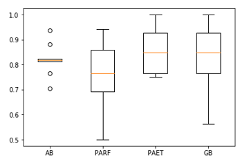
Figure 1:  Ensemble algorithms’ performance

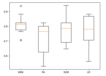
Figure 2:  Algorithms performance

• In Figure 4 the size of estimators is examined for the ensemble performance (Figure 4). Three models are used in the experiment: PABAG, PARF, PAET. The Breast Cancer Wisconsin dataset (BCWD) from UCI site is used. The accuracy of each method over various numbers of estimators using a 10-fold cross validation is examined. All methods tend to perform similarly and yield high accuracies for over 10 estimators.
• In Figure 5 for the base estimator (decision tree), which is common for the three models, the tree depth is the most important measure of complexity since deeper trees are more complex. In Figure 5 the complexity of the models against the performance using the depth of the base decision trees is examined. Again here, a 10-fold cross validation shows average performance values in all tested methods over various maximum depths. All three methods tend to yield high accuracy values over all chosen depths but all of them obtain their best accuracies at a depth equal to 8. In general, we see that PABAG tends to yield larger accuracies over all other methods for various depths.
• In Figure 6 learning rate using XGBoost (boosting algorithm) for defining the appropriate rate for the performance. Cross Validation is used to set the learning rate. The XGBoost degrades the performance as the boosting process exhibits the overfitting behavior. From Figure 6 the value of 1.2 or any value between 1.0 and 1.5 could be appropriate.
• In figure 7 control technique to stop the training with XGBoost. The accuracy is improving while the XGBoost continues training. When there is not any improvement of accuracy XGBoost terminates the training. In this way, the process terminates in a round which will be less than the predefined number of iterations. The training stops when the accuracy has better value after the next five rounds, From Figure 7 it is the 32 rounds when the training stops since the next five values are less than the one of 32 round (0.993449).

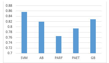
Figure 3: Accuracy with SVM and ensemble models

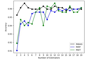
Figure 4: Performance vs Size of Estimators

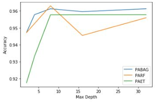
Figure 5:  Accuracy vs Depth of trees in Ensemble

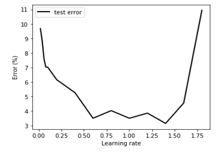
Figure 6:   Learning rate discovery

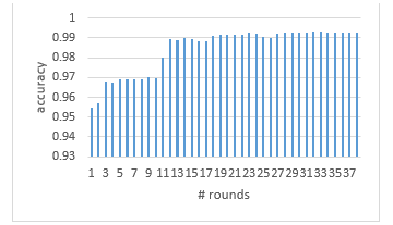
Figure 7: Accuracy vs # of rounds

10.  Conclusion

Tree-based ensembles are considered state-of-the-art. The augmentation of the prediction power using individual algorithms or tree-ensemble models and their internal composition is an open issue. For this purpose, PA has been developed as the base model for the proposed ensemble since it avoids the replication problem of DTs by using the CNN criterion.

Ensemble learning helps improve overall accuracy by combining the results from several models. These models are known as weak learners trained to solve the same problem while their combination leads to more accurate and robust models. The kNN surpasses PA, SVM and LR. AB outperforms PARF, PAET, and GB. The SVM with the polynomial kernel exceeds even the ensemble models. Higher accuracy is achieved by an appropriate algorithm rather than ensemble models.

From the comparison of the two sets of algorithms the selection of models with their hyperparameters for creating an ensemble model could be an issue if other algorithms with their tuning parameters can provide good performance. The ensemble size and the depth of the trees affect the performance of the model. For boosting ensemble, the best learning rate with the use of XGBoost allows a good training strategy for the creation of the appropriate model. A reactive approach for terminating the training time by enforcing early stopping is also achieved.

Future work could be based on the stacking of heterogenous ensemble models.

1. J. Tsiligaridis, “Tree-Based Ensemble Models and Algorithms for Classification”, in 2023 International Conference on Artificial Intelligence in Information and Communication (ICAIC 2023),103-106, 2023, doi: 10.1109/ICAIIC57133.2023.10067006
2. J. Han, M. Kamber, J. Pei, “Data Mining Concepts and Techniques”,Morgan Kaufman, 2012
3. M.Karntardzic,“Data Mining: Concepts, Models, Methods, and Algorithms”, IEEE Press, 2003.
4. L. Rokach, O. Maimon, ”Data Mining with Decision Trees”. World Scientific , 2008
5. I. Nti, A. Adekoya, B. Weyon, “A comprehensive evaluation of ensemble learning for stock-market prediction” , Journal of Big Data , 7(1), 1-40, 2020, doi: 10.1186/s40537-020-00299-5
6. W. Yu, T. Liu, R. Valdez, M. Gwinn, M. Khoury, “ Application of support vector machine modeling for predictiion of common diseases: the case of diabetes and pre-diabetes”, BMC Medical Informatics and Decision Making, 10(1): 16, 2010, doi: 10.1186/1472-6947-10-16
7. S. Huang, N. Cai, P. Pacheco, S. Narandes, Y. Wang, W. Xu, “Applications of Support Vector Machines (SVM) Learning in Cancer Genomics”, Cancer Genomics&Proteomics,Journal,15(1),41-51,2018, doi: 10.21873/cgp.20063
8. R. Couronne, P. Probst, A. Boulesteix, “Random Forest versus Logistic Regression: a large-scale benchmark experiment”, BMC Bioinformatics, 19, 270, 2018, doi: 10.1186/s12859-018-2264-5
9. E.K. Ampomah, Z. Qin, G. Nyame, “Evaluation of tree-based Ensemble Machine Learning Models in predicting Stock Price Direction of Movement”, Information Journal, MDPI, 11(6), 332, 2020, doi:10.3390/info11060332
10. A. Zafari, R. Zurita-Milla, E. Izquierdo-Verdiguier, “Land Cover Classification Using Extremely Randomized Trees: A Kernel Perpective” IEEE Geoscience and Remote Sensing Letters,17(10),1702-1706, 2020, doi: 10.1109/LGRS.2019.2953778.
11. L. Li, J. Qiao, G. Yu, L. Wang, H. Li, C. Liao, Z. Zhu, “Interpretable tree-based ensemble model for predicting beach water qaulity”, Water Research, 211, 118078, 2022, doi:10.1016/j.watres.2022.118078
12. M. Jaxa-Rozen, J. Kwakkel, “Tree-based ensemble methods for sensitivity analysis of environmental models: A performanced comparison with Sobol and Morris technique”, Science Direct, 107, 245-266, 2018 doi:10.1016/j.envsoft.2018.06.011
13. P.Han, M.Steinbach, A. Karpatne, V. Kumar, ”Introduction to data Mining”,Pearson, 2019
14. A. Geron, “Hands On Machine Learning with Scikit-Learn & Tensorflow”,O’REILLY,2017
15. J.Gareth, D. Witten, T. Hastie, R. Tibshirani, “.An Introduction to Statistical Learning with Applications in R”, Springer, 2017
16. L.Rokach,”Ensemble Learning: “Patern Classification Using Ensemble Methods”, World Scientific, 2009
17. R. Natras, B.Soja, M. Schmidt, “ Ensemble Machine Learning of Random Forest, AdaBoost, and XGBost for Vertical Total Electron Content Forecasting ”, Remote Sensing, MDPI, 14(15), 3547, 2022 doi:10.3390/rs14153547
18. M.Ramakrisna,V.Venkatesan,I Izonin, M.Havryliuk, C.Bhat, “Homogenous Adaboost Endemble Machine Learning Algorithms with Reduced Entropy on Balanced Data”, Entropy, MDPI, 25, 245,2023, doi:10.3390/e25020245
19. B. Kalaiselvi, S. Geetha, “Ensemble Machine Learning AdaBoost with NBtree for Placement Data Analysis”, in 2nd International Conference on Intelligent Technology (CONIT) , 1-4 , 2022, doi: 10.1109/CONIT55038.2022.9847993
20. Sonar dataset: http://archive.ics.uci.edu/ml/datasets/connectionist+bench+(sonar,+mines+vs.+rocks)

(Click Here)