1. Introduction

In the past several years, convolutional neural networks (CNNs) have been used to solve issues in the disciplines of computer vision and medical image analysis.  By now, deep learning-based image segmentation has gained a solid reputation as a reliable technique for picture segmentation. As the initial and crucial step in the pipeline for diagnosis and treatment, it has been routinely employed to divide homogeneous areas [1]. Today, many people experience illness, including cancer. Brain tumors can be either benign or malignant. A brain tumor is an enlargement of brain cells or cells close to the brain. Brain tissue can give rise to brain tumors. The membranes that encircle the surface of the brain, the pituitary gland, and the pineal gland are neighboring structures. An unchecked cell proliferation that threatens the central nervous system’s survival is known as a brain tumor. Primary and secondary brain cancers fall into separate categories. Primary brain malignancies begin in brain cells, as opposed to secondary cancers, which spread to the brain from other organs. Primary brain tumors are gliomas. High-grade glioblastoma (HGG) and low-grade glioblastoma (LGG) are two more kinds of gliomas. The results of brain tumor segmentation can be utilized to generate quantitative measurements for glioblastoma diagnosis and treatment planning. Segmenting 3D modalities is a difficult task involving deviations and errors, in contrast to radiologists manually evaluating MRI modalities to gain quantitative information. [2]. In the medical industry, segmenting an image into its component components to extract features is a crucial task. Picture segmentation, which often comprises semantic segmentation and instance segmentation, is a significant challenge in the study of computer vision (CV).

Multimodal Brain Tumor Image Segmentation (BRATS), a yearly workshop and competition, has been held in recent years to compare several benchmark techniques created to segment the brain tumor [3]. In clinical contexts, common standard imaging modalities include ultrasound, magnetic resonance imaging (MRI), and computed tomography (CT). Because the multiple image contrasts of these MRI protocols can be used to extract crucial supplemental information, numerous prior studies have demonstrated that multimodal MRI protocols can be used to identify brain cancers for treatment planning. T2-weighted fluid-attenuated inversion recovery (FLAIR), T1-weighted (T1), T1-weighted contrast-enhanced (T1c), and T2-weighted (T2) are among the multimodal MRI techniques. Variations in the organs’ size, location, and shape make this problem more challenging. Convolutional Neural Networks (CNNs) can, however, be utilized to develop automatic segmentation techniques using MRI data [4], [5]. Deep learning algorithms produce more robust features than conventional discriminative models based on pre-defined features because they learn a hierarchy of progressively more complex task-specific features directly from the data. Deep CNNs have produced outstanding results for segmenting brain tumors [6]-[14].  In this work, we aim to segment Tumor brain MRI volumes. Due to the many appearances the tumor brain can take on in several scans because of deformations and variations in the intensity distribution, this is a difficult assignment. Moreover, due to field inhomogeneity, MRI volumes are frequently impacted by artifacts and distortions. One of the primary problems with brain lesion identification is that, because lesions only affect a small portion of the brain, unsophisticated training algorithms are more likely to choose the pointless choice of null detection. and therefore can extract the features of the three regions with greater accuracy. As a result, it has produced impressive results and made outstanding contributions to the clinical diagnosis and care of patients with brain tumors [15]. There are a lot of studies involving deep learning techniques and explaining them in details [16]-[18]. All instances of a class are found using instance segmentation, with the added ability to distinguish between distinct instances of any segment class[19]. Segmentation method entered in many medical and biological specialties [20],[21].Tumor brain segmentation interesting task to many author [22], [23]. Deep learning important technique for many applications [24].

2. Related work

The researcher In this study [5], They employed ROI masks to restrict the networks’ training to relevant voxels and a cascade of two CNNs, inspired by the V-Net design, to segment brain tumors. This architecture facilitates dense training on problems with highly skewed class distributions, such as brain tumor segmentation, by limiting training to the vicinity of the tumor area. The results are based on data from the BraTS2017 Training and Validation sets. In this paper [13], For the segmentation of 3D images, they suggested a volumetric, fully convolutional neural network-based approach. After being trained from beginning to end on MRI volumes of the prostate, the network learns to predict segmentation for the full volume at once. This work introduces an objective function that optimizes during training and is based on the Dice coefficient. They deal with situations where the number of foreground and background voxels differs significantly. Histogram matching and random non-linear adjustments were utilized to augment the data and compensate for the minimal number of annotated volumes that were available for training. In this paper [14]  suggested the AGSE-VNet framework for automatically segmenting MRI data from brain tumors. Using the channel relationship, the Squeeze and Excite (SE) module and Attention Guide Filter (AG) module are used to automatically enhance the useful information in the channel and suppress the useless information, and the attention mechanism is used to guide the edge detection and eliminate the influence of irrelevant information. Utilizing the online verification tool for the BraTS2020 challenge, results have been analyzed. Verification focuses on the fact that the Dice scores for the whole tumor (WT), tumor core (TC), and enhanced tumor (ET) are, respectively, 0.68, 0.85, and 0.70. Conclusion Despite the fact that MRI images have varying intensities, AGSE-VNet is unaffected by the tumor’s size and therefore can extract the features of the three regions with greater accuracy. As a result, it has produced impressive results and made outstanding contributions to the clinical diagnosis and care of patients with brain tumors. In this [15] the researcher used 2D V-net K for tumor brain segmentation and enhancing predication they used data set BRATS2020.

3. Materials and Methods

3.1.  Segmentation

The term “image” refers to a matrix of pixels that are ordered in rows and columns according to coordinates. There are numerous methodologies for constructing an image, including enhancement, detection, compression, segmentation, and more. As an alternative, segmentation is the act of labeling pixels.. Image segmentation is a technique used in the field of image processing that divides a digital image into several subgroups known as “image segments,” which functions to simplify prospective processing or interpretation of the image by reducing the complexity of the original image. There is a distinct name for each pixel or component of a picture that belongs to the same category.   Semantic segmentation, instance, and panoptic segmentation, are three prominent type of segmentation as shown in figure1.

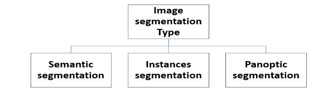
Figure 1: Show the approach of Image segmentation.

One of the most challenging problems in computer vision, particularly in medical image analysis, is semantic segmentation, the act of giving a class label to each pixel. Semantic segmentation helps with the automatic localization and detection of sick structures.[16], Semantic segmentation aims to classify different areas of a picture into categories. The segment could be viewed as a categorization issue at low resolution. Segmentation is used in computer-aided diagnosis to extract anatomical sections and has been a significant research area for information extraction[17]. When utilizing deep learning for semantic segmentation, the learning process is supervised and the training images containing actual classes that have been separated, also known as ground truth data, are connected to the labels. Semantic segmentation is used in numerous industries, including the medical sector.

When numerous instances are combined into one class, the problem description is frequently ambiguous when utilizing this approach. For example, the “people” class may be used to classify the entire crowd in a bustling scene. The semantic segmentation does not provide enough detail for this complex image.

Instance segmentation is a specific type of picture segmentation that focuses on locating instances of objects and defining their bounds. Instance segmentation has drawn interest in several computer vision disciplines, including autonomous vehicle control, drone navigation, and sports analysis. Numerous effective models have recently been created, and they can be divided into two groups: speed-focused and accuracy-focused. For this task to be used in real-time applications, accuracy and inference time are crucial.[19]. Thus, semantic segmentation differs from instance segmentation in that it treats many objects belonging to the same category as a single entity. As opposed to that, instance segmentation detects specific objects within  the image[20].

Panoptic segmentation the most current segmentation task, known as panoptic segmentation, can be described as a combination of instance and semantic segmentation, where each instance of an object in the image is separated and its identification is foreseen. Popular activities like self-driving automobiles, where a significant amount of information about the immediate surroundings must be gathered with the aid of a stream of photos, find widespread application for panoptic segmentation algorithms. In figure2 [18] show the panoptic, semantic and instance segmentation.

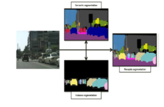
Figure 2: Demonstrate how instance segmentation, semantic segmentation, and panoptic segmentation vary from one another.

The segmentation technique belongs to the class of pixel cases. The first approach makes use of discontinuity to segment an image into lines, edges, and isolated points by identifying them based on rapid changes in local properties. The regions’ boundaries are then deduced. By utilizing the homogeneity of spatially dense information, such as texture, intensity, and color, the second method’s segmentation results are generated. The third strategy combines boundary-based segmentation and segmentation based on regions.  [3]. Most current tumor segmentation techniques can be grouped into one of two big families based on how they segment tumors. The main drawback with image segmentation is over segmentation and high sensitivity to noise. Discriminative techniques focus on select local picture features that seem significant for the tumor segmentation job, directly learning the link between image intensities and segmentation labels without any domain knowledge. The most important picture segmentation techniques include threshold-based, edge-based, region-based, clustering-based, and “deep learning” based on artificial neural networks (3). Model training is used in machine learning-based image segmentation approaches to enhance the system’s capacity to recognize key traits. For photographic segmentation tasks, deep neural network technology is highly effective.

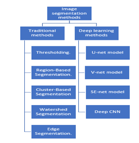
Figure 3: Show the traditional segmentation methods and deep learning methods

3.2.  Deep learning methods with segmentation approach

Artificial neural networks, which are the sole foundation of the machine learning subfield of deep learning, will replicate the human brain in a manner like how neural networks do for deep learning. Because Deep Learning models can dynamically learn features from the input, they are ideal for applications like photo recognition, speech recognition, and natural language processing. The three most widely used deep learning designs are feedforward neural networks, convolutional neural networks (CNNs), and recurrent neural networks (RNN). A feedforward neural network (FNN), which has a linear information flow, is the most fundamental type of ANN. FNNs have been widely employed for tasks such as image classification, image segmentation, speech recognition, and natural language processing. Convolutional neural networks (CNNs) that were trained on manually labeled patient datasets are the foundation of most contemporary automatic segmentation methods. For image segmentation, a variety of neural network implementations and architectures are suitable. They frequently share the same essential components. An encoder is a group of layers that uses more specific, in-depth filters to extract visual characteristics. By using its earlier experience with a task that is comparable to this one (like image recognition), the encoder may be able to carry out segmentation tasks. A decoder is a collection of layers that gradually transforms the encoder’s output into an interpretation according to the pixel resolution of the input image. To enhance model accuracy, skip connections. Multiple long-range neural network connections that let the model recognize significant information at many scales are used. There are many models used to segment images; the most famous and important are U-net models[21] segment for biomedical image , V-net models [13] segment for volume medical image in follow section more description for each one.

a.       V-net model:

The [13] proposed On both the left and right sides of the V-Net, there are many layers. The network’s right and left halves alternately decompress and compress the signal until it is back to its original size. The network’s left side is divided into several stages, each of which can operate in a different configuration. Each phase has between one and three convolutional layers. Each level involves the learning of a residual function. Each step’s input is applied to its respective convolutional layers, subjected to non-linear processing, and added to the output of the final convolutional layer to enable the learning of a residual function. Comparison of this design to non-residual learning networks like U-Net ensures convergence.

The volumetric kernels used in each stage’s convolutions have a 5x5x5 voxel size. (A voxel in 3D space corresponds to a value on a standard grid. Like how “voxelization” is used in point clouds, the word “voxel” is widely employed in 3D spaces.) The resolution of the compression path is decreased by stride 2 convolution using 2x2x2 voxel wide kernels. As a result, the objective of layer pooling is still accomplished while halving the size of the generated feature maps. The number of feature channels doubles at each stop along the V-compression Net’s journey. Convolutional operations have a smaller memory footprint during training because they do not need switches to change the output of pooling layers back to their inputs for back-propagation. sampling backwards. They leave a lower memory footprint when training. It is possible to expand the receptive field by downsampling. A nonlinear activation function is employed with PReLU.

The network extracts feature from the lower resolution feature maps, enhances the spatial support for those features, and collects the required data to construct a two-channel volumetric segmentation. In each step, the inputs are deconvolved to increase their size, and then one to three convolutional layers are added, each of which uses half as many 5x5x5 kernels as the layer before it. Residual function is taught, just like in the left part of the network.

The output size of the final convolutional layer, which has a 1x1x1-kernel size, is the same as the input volume. The two feature mappings are generated. With the use of soft-max voxel-wise segmentation, these two output feature maps provide probabilistic foreground and background segmentations. lateral connections Similar to U-Net, compression results in the loss of location data (left). As a result, horizontal connections are used to transfer the features that were acquired from the left part of the CNN’s first stages to the right part.  By doing so, better precision of the final contour forecast and the correct part position data have been achieved. The model’s convergence is accelerated by these linkages. Figure 4 shows the structure of V-net.

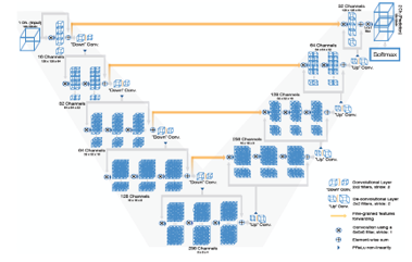
Figure 4: Show the structure of V-net [13]

b.       U-net model:

The U-net model is a significant model that includes biomedical imagery. [21], take U shape as shown in figure 4. [21] it’s have three part encoder, decoder and bottleneck. For classification-related issues, the tool that turns an image into a vector that can be used for classification is useful. However, in order to segment a picture, the feature map must also be turned into a vector, which must then be used to recreate the original image. This is a hard operation because it is far more difficult to convert a vector into a picture than the contrary, this is the main issue with U net-design. The three components of the U-net model are contraction, bottleneck, and expansion. In the U-Net model, the contraction is employed to expand a vector into a segmented image. This would preserve the structural integrity of the image and significantly lessen distortion.

The architecture can successfully learn the complex structures since there are twice as many kernels or feature maps after each block. A mediator between the contraction layer and the expansion layer is the bottom layer. After two 3X3 CNN layers, a 2X2 up convolution layer is applied.

The number of blocks for both expansion and contraction is the same. Yet, the extension component is where this architecture’s core may be located. Several expansion building elements are included in addition to the contraction layer. A 2X2 up sampling layer is added to each block after the first two 3X3 CNN layers to handle the input. To maintain symmetry, the convolutional layer uses half as many feature mappings between each block. But each time, the input is also supplemented by feature maps from the associated contraction layer. As a result, the traits identified during the image’s contraction would be considered during its reconstruction. The subsequent 3X3 CNN layer receives the output mapping, with the number of feature mappings matching the necessary number of segments. This model, U-net, has been used with the 2018 Brast data set in this paper to evaluate the optimization of V-net, as shown in Figure 6.

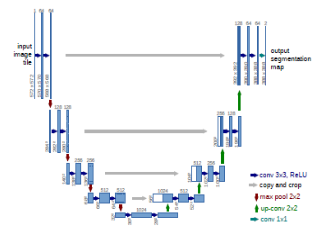
The figure 5: Show the U-net model

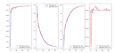
Figure 6: Show the training of U-net model with 2018Brast.

3.3.   Attention 2D-layer.

Deep learning approaches such as attention models or attention mechanisms are used to add additional focus to a particular component. Focusing on something special and noting its unique value is what deep learning is all about. The attention mechanism was first made available by[24]. To address the bottleneck problem brought on by a fixed length encoding vector, where the decoder’s access to the input’s data would be severely limited. Because the representation’s dimensionality would be limited to match that of shorter or simpler sequences, this is seen to be especially troublesome for long and/or complex sequences.

The attention layer’s goal is to increase the machine translation encoder-decoder model’s effectiveness. By integrating all the encoded input vectors in a weighted fashion, with the most pertinent vectors receiving the highest weights, the attention mechanism was developed to enable the decoder to use the most pertinent sections of the input sequence in a flexible manner.

As indicated in the findings section, the attention layer and V-net model were integrated in this study to increase training effectiveness. As seen in figure 7, the attention layer used in this study is composed of a convolution layer followed by Relu activation, convolution, followed by a sigmoid function.

Boost helpful functions and disable less helpful ones for the present work. The image is decompressed after each decoder receives the down sampling characteristics for the corresponding step. In the process of downsampling, the attention block is used to remove background noise and unnecessary details, while the image filter (edge information) directs the structural and feature data for the images. Remember that the model uses the skip connection idea to prevent gradient vanishing.

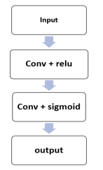
Figure 7: Show the structure of attention layer.

4. Proposed Method

Encoder and decoder components are symmetrical in the network’s structure. The encoder is made up of four blocks, each of which contains several convolution layers, batch normalization, and PRelue. Between each block, there is a Max pooling layer with (2,2), which allows for down sampling and equivalent up sampling. All convolution layers have size 5x5with stride [1,1]. A full skip connection is joined with concatenation to keep the feature map and resolution of the image. Using skip connections following sampling at the decoding end, the lower-level features are fused with the first four scales of the feature map of the V-net.

Four blocks make up the decoder side, including an attention layer with a kernel size of (1,1) and a stride of 1. The layer’s first three operations are convolution, relu activation, and sigmoid.   Encoding equipment Batch normalization facilitates weight initialization and speeds up network training by enabling significantly higher learning rates. While building deeper networks, initializing weights might be challenging. The addition of a 2D attention layer can enhance this model. Many researcher worked on V- net model and  optimized it [5,14]. The optimize in this research was by adding attention layer with encoder. There are full skip connections between encoder and decoder.

This model V-net makes use of the Brast 2018 data set to produce feature maps with modest values but concentrated, high-dimensional semantic interpretations after continuous convolution. To provide a segmentation result, the decoder is then repeatedly convolved and up sampled to the original size.

By batch normalizing, the sensitivity to the original beginning weights is reduced. To utilize a suitable stride at the conclusion of each block to reduce its resolution. The network’s left side compresses the signal while the right side decompresses it until the signal’s original size is reached.[13].

4.1.  Evaluation criteria

To Evaluate this work, we need take in our consideration many criteria. We gauge the training of our model using the loss, accuracy, mean IOU, dice coefficient, precision, sensitivity, and specificity.

a.         Loss function:  A loss function compares the target and anticipated output values to determine how well the neural network mimics the training data. During training, we make an effort to minimize this difference between the expected and desired outputs. determined by.

1. Accuracy: Accuracy is a measure of the model’s performance across all classes. It is useful when all classes are given equal weight. It is calculated as the ratio of events that were successfully anticipated to all events that were predicted. One of the measures that is most frequently used when performing categorization is accuracy.. We explain each term in table 1.

Tabel.1: Describe the criteria for validity.
	A true positive result is one that the model correctly identified as falling within the positive category.
	When the model correctly predicts the negative class, the result is said to be True Negative.
	False Negative: is a finding when the model forecasts the positive class wrongly.
	False Negative: is a outcome genuine positive instances are labeled as negative

1. Mean IOU: mean intersection over union is used when calculating mean average precision.

1. Dice coefficient: A predicted segmentation’s pixel-by-pixel agreement with the associated ground truth can be compared using the Dice coefficient. In image segmentation, the Dice score coefficient is a commonly used metric of overlap. The benefit of dice loss is that it does a good job of handling the class mismatch between the foreground and background pixel counts.

1. Precision: One indicator of the model’s performance is precision, or the quality of a successful prediction the model makes. By dividing the total number of positive predictions by the percentage of true positives, precision is determined (i.e., the number of true positives plus the number of false positives).

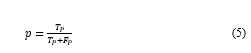
1. Sensitivity: One indicator of the model’s performance is precision, or the quality of a successful prediction the model makes. By dividing the total number of positive predictions by the percentage of true positives, precision is determined.

1. Specificity: The fraction of true negatives that the model correctly predicts is known as specificity. Specificity can be defined as the ability of the algorithm or model to predict a genuine negative of each possible category. It is sometimes referred to as the genuine negative rate in literature.

4.2.  Descriptive for Data Set

The three sources for the BraTS 2018 challenge are indicated, respectively, by the designations “2013,” “CBICA,” and “TCIA.” The training data set contains 20 cases of high-grade glioma (HGG) from the 2013 group, 88 cases from CBIC, and 102 cases from TCIA, as well as 10 cases from 2013 and 65 cases from TCIA participants who had low-grade gliomas (LGG), which are less active and infiltrative. [22] .One of dataset that is frequently used in the world of healthcare is BRATS 2018 which used in this paper include tow folder HHG and LLG each one has 2oo case patients we used 55 cases in this paper.

Per case, BRATS provides four multimodal MRI modalities. The four MRI modalities that the BRATS competition organizers provide, along with associated manual segmentation, include 3D brain MRIs with ground truth brain tumor segmentations annotated by physicians (T1, T1c, T2, and FLAIR): T1-weighted (T1), T1-weighted post-contrast (T1c), T2-weighted (T2), and fluid-attenuated inversion recovery (FLAIR). [6]. The link of data set; which used in this paper BRAST2018 can find on this     https://www.kaggle.com/datasets/sanglequang/brats2018/download?datasetVersionNumber=10.

The volume dimension of every MRI in the BRATS 2018 dataset is 240 x240 x155. The data set which used in this study MRI 3D image (voxel) tumor brain which represented by X, Y, Z, 3D, non-informative voxels are found in medical images in general and brain MRIs. The preprocessing with this data started by converted the voxel to pixel it’s mean 3D to 2D image to reduce the consuming time. The HGG have be used in this article have four modalities (T1, T1c, T2, and FLAIR). The data set in this paper divided to training and test, the test split to test and validation. The size of training is 2970 with dimension (192X192X4), and the size of test and validation is 990 with dimension (192X192X4). It is difficult to discern between a tumor and normal tissue despite the fact that tumor margins are typically fuzzy and that there is a considerable deal of variation in shape, location, and expression among patients. Despite recent developments in automated algorithms, segmenting brain tumors in multimodal MRI scans remains a difficult task in medical image processing [5]. The biggest obstacle to segmenting brain tumors is the class imbalance. Even less of the brain’s tissue between 5 and 15% represents each tumor site [23].

5. Result and discussion

We improved and suggested V-Net-attention 2D based fully convolutional networks to address the brain tumor segmentation challenge. In essence, semantic segmentation is the task that deals with tumor recognition and segmentation. The data set of BRAST2018 divided to training, validation and test set with 35 epochs and the size of batch 8, because high memory consumption is still challenge in 3D-CNNs. The developed model was implemented on colab and evaluated on brain magnetic resonance images MRI. The findings demonstrate that this proposed technique outperforms several of the already popular derivative models based on CNNs in terms of segmentation performance and tumor recognition accuracy. The experiment started by pre-processing to data set, input slice of the BRAST dataset which feed to model have dimension 192x192x4 (h x w x d, refereed to Hight, width and depth respectively) in this paper. In comparison to earlier deep learning-based studies on this subject, we train U-net on the same BRAST2018 data set as indicated in the preceding section. The results reveal that training improves V-net by adding an attention layer, which has a decent performance on HGG as show in figure8. Take optimizers Adam with learning rate (lr=1e-5).

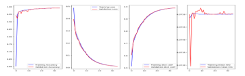
Figure 8: Show the training of V-net attention 2D on the HGG.

The measurement of classification accuracy as well as localization correctness is thought to be required in the analysis of semantic segmentation, which can be complex. The objective is to evaluate how closely the predicted (prediction) and annotated segmentation differ (ground truth). We used different benchmark to evaluate the optimized model V-net Attention 2D where take in consideration loss, Accuracy, Mean_IOU, dice_coef, precision, sensitivity, specificity demonstrated in table2, Instead, it is a helper metric that assesses the level of agreement between the ground truth and prediction.

Table 2: Show the result through training of model V-net attention 2D.

	loss	accuracy	MeanlOU	Dice_coef	precision	sensitivity	specificity
Train result	0.0105	0.99203	0.37501	0.9894	0.9926	0.99156	0.99754
Validation result	0.0108	0.99174	0.37502	0.9891	0.9923	0.99128	0.99744
Test result	0.0107	0.99175	0.37501	0.9892	0.9924	0.99124	0.99747

Here, we improve a strategy for segmenting medical pictures using fully convolutional neural networks that have been end-to-end trained to locate tumors in MRI scans. In contrast to previous recent techniques, Convolutions and BRAST 2018’s slice-wise input volume processing are recommended. One of the primary issues with tumor brain is that since these lesions only impact a small portion of the brain, simple training methods are predisposed to the useless option of null detection. Only brain tissue will be used to train the modified V-NET first network model to produce raw data and predict the normal region, as shown in figure 9.

6. Conclusion

In the study developed a deep convolution network-based, fully automatic method for locating and classifying brain cancers in this study. Through tests on a well-known benchmarking dataset (BRATS 2018), which covers both HGG and LGG patients, we have demonstrated that our method can deliver both efficient and robust segmentation relative to manually determined ground truth. Our V-Net 2D attention-based deep convolution networks may also yield outcomes that are comparable for the overall tumor region and even better for the core tumor region when compared to existing state-of-the-art methods. The presented method can be used to generate a patient-specific brain tumor segmentation model without the requirement for manual assistance, which might enable objective lesion assessment for clinical tasks like diagnosis, treatment planning, and patient monitoring.

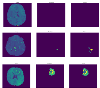
Figure 9: Illustration of the V-net-Attention 2D for normal cases HGG segmentation results in BraTS2018.

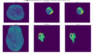
Figure 10: Demonstration of the V-net-Attention 2D segmentation findings for cases of brain tumors and brain tissue from BraTS2018.

Acknowledgment

The accomplishment of this study was supported by a grant from the institution Moscow Institute of Physics and Technology.

1. M.H. Hesamian, W. Jia, X. He, P. Kennedy, “Deep Learning Techniques for Medical Image Segmentation: Achievements and Challenges,” Journal of Digital Imaging, 32(4), 582–596, 2019, doi:10.1007/s10278-019-00227-x.
2. P. Ahmad, S. Qamar, L. Shen, A. Saeed, “Context Aware 3D UNet for Brain Tumor Segmentation,” Lecture Notes in Computer Science (Including Subseries Lecture Notes in Artificial Intelligence and Lecture Notes in Bioinformatics), 12658 LNCS, 207–218, 2021, doi:10.1007/978-3-030-72084-1_19.
3. B.H. Menze, A. Jakab, S. Bauer, J. Kalpathy-Cramer, K. Farahani, J. Kirby, Y. Burren, N. Porz, J. Slotboom, R. Wiest, L. Lanczi, E. Gerstner, M.A. Weber, T. Arbel, B.B. Avants, N. Ayache, P. Buendia, D.L. Collins, N. Cordier, J.J. Corso, A. Criminisi, T. Das, H. Delingette, Ç. Demiralp, C.R. Durst, M. Dojat, S. Doyle, J. Festa, F. Forbes, et al., “The Multimodal Brain Tumor Image Segmentation Benchmark (BRATS),” IEEE Transactions on Medical Imaging, 34(10), 1993–2024, 2015, doi:10.1109/TMI.2014.2377694.
4. H.T. Le, H.T. Thu Pham, “Brain tumour segmentation using U-Net based fully convolutional networks and extremely randomized trees,” Vietnam Journal of Science, Technology and Engineering, 60(3), 19–25, 2018, doi:10.31276/vjste.60(3).19.
5. A. Casamitjana, M. Catà, I. Sánchez, M. Combalia, V. Vilaplana, “Cascaded V-Net using ROI masks for brain tumor segmentation,” Lecture Notes in Computer Science (Including Subseries Lecture Notes in Artificial Intelligence and Lecture Notes in Bioinformatics), 10670 LNCS, 381–391, 2018, doi:10.1007/978-3-319-75238-9_33.
6. M. Ghaffari, A. Sowmya, R. Oliver, “Automated Brain Tumour Segmentation Using Cascaded 3D Densely-Connected U-Net,” Lecture Notes in Computer Science (Including Subseries Lecture Notes in Artificial Intelligence and Lecture Notes in Bioinformatics), 12658 LNCS, 481–491, 2021, doi:10.1007/978-3-030-72084-1_43.
7. H. Dong, G. Yang, F. Liu, Y. Mo, Y. Guo, “Automatic brain tumor detection and segmentation using U-net based fully convolutional networks,” Communications in Computer and Information Science, 723, 506–517, 2017, doi:10.1007/978-3-319-60964-5_44.
8. Q. Jia, H. Shu, “BiTr-Unet: A CNN-Transformer Combined Network for MRI Brain Tumor Segmentation,” Lecture Notes in Computer Science (Including Subseries Lecture Notes in Artificial Intelligence and Lecture Notes in Bioinformatics), 12963 LNCS, 3–14, 2022, doi:10.1007/978-3-031-09002-8_1.
9. A. Atiyah, K. Ali, “Brain MRI Images Segmentation Based on U-Net Architecture,” Iraqi Journal for Electrical and Electronic Engineering, 18(1), 21–27, 2022, doi:10.37917/ijeee.18.1.3.
10. V.P. Gladis Pushpa Rathi, S. Palani, “Brain tumor detection and classification using deep learning classifier on MRI images,” Research Journal of Applied Sciences, Engineering and Technology, 10(2), 177–187, 2015.
11. M.A. Al Nasim, A. Al Munem, M. Islam, M.A.H. Palash, M.M.A. Haque, F.M. Shah, “Brain Tumor Segmentation using Enhanced U-Net Model with Empirical Analysis,” 2022.
12. K. Munir, F. Frezza, A. Rizzi, “Deep Learning Hybrid Techniques for Brain Tumor Segmentation,” Sensors, 22(21), 2022, doi:10.3390/s22218201.
13. F. Milletari, N. Navab, S.A. Ahmadi, “V-Net: Fully convolutional neural networks for volumetric medical image segmentation,” Proceedings – 2016 4th International Conference on 3D Vision, 3DV 2016, 565–571, 2016, doi:10.1109/3DV.2016.79.
14. X. Guan, G. Yang, J. Ye, W. Yang, X. Xu, W. Jiang, X. Lai, “3D AGSE-VNet: an automatic brain tumor MRI data segmentation framework,” BMC Medical Imaging, 22(1), 2022, doi:10.1186/s12880-021-00728-8.
15. D. Rastogi, P. Johri, V. Tiwari, “Brain Tumor Segmentation and Tumor Prediction Using 2D-VNet Deep Learning Architecture,” Proceedings of the 2021 10th International Conference on System Modeling and Advancement in Research Trends, SMART 2021, (August 2022), 723–732, 2021, doi:10.1109/SMART52563.2021.9676317.
16. Y. Azzi, A. Moussaoui, M.-T. Kechadi, “Semantic Segmentation of Medical Images with Deep Learning: Overview,” Medical Technologies Journal, 4(3), 568–575, 2020, doi:10.26415/2572-004x-vol4iss3p568-575.
17. J. Moorthy, U.D. Gandhi, “A Survey on Medical Image Segmentation Based on Deep Learning Techniques,” Big Data and Cognitive Computing, 6(4), 2022, doi:10.3390/bdcc6040117.
18. O. Elharrouss, S. Al-Maadeed, N. Subramanian, N. Ottakath, N. Almaadeed, Y. Himeur, “Panoptic Segmentation: A Review,” 2021.
19. S. Jung, H. Heo, S. Park, S.U. Jung, K. Lee, “Benchmarking Deep Learning Models for Instance Segmentation,” Applied Sciences (Switzerland), 12(17), 1–25, 2022, doi:10.3390/app12178856.
20. T. Scherr, A. Bartschat, M. Reischl, J. Stegmaier, R. Mikut, “Best Practices in Deep Learning-Based Segmentation of Microscopy Images,” Proceedings – 28. Workshop Computational Intelligence, Dortmund, 29. – 30. November 2018. Ed.: F. Hoffmann, 175, 2018.
21. T.B. Olaf Ronneberger, Philips Fischer, “U-Net: Convolutional Networks for Biomedical Image Segmentation,” IEEE Access, 9, 16591–16603, 2015, doi:10.1109/ACCESS.2021.3053408.
22. L. Dai, T. Li, H. Shu, L. Zhong, H. Shen, H. Zhu, “Automatic Brain Tumor Segmentation with Domain Adaptation,” 1–12, 2018.
23. L.M. Ballestar, V. Vilaplana, “MRI Brain Tumor Segmentation and Uncertainty Estimation Using 3D-UNet Architectures,” Lecture Notes in Computer Science (Including Subseries Lecture Notes in Artificial Intelligence and Lecture Notes in Bioinformatics), 12658 LNCS(1), 376–390, 2021, doi:10.1007/978-3-030-72084-1_34.
24. D. Bahdanau, K.H. Cho, Y. Bengio, “Neural machine translation by jointly learning to align and translate,” 3rd International Conference on Learning Representations, ICLR 2015 – Conference Track Proceedings, 1–15, 2015.

(Click Here)