1. Introduction

This paper extends our previous work presented in CCECE 2022 [1] underwater signal processing. Sonar systems, particularly underby introducing a selective-modal algorithm architecture for localizwater sonars, have undergone rapid developments in the past two ing impulsive sound sources in shallow waters. Our proposed algodecades, driven by increased processing capability and the implerithm improves performance in lower signal-to-noise ratio (SNR) mentation of more computationally intensive techniques. The underscenarios by selecting the best modal pairs. In this paper, we provide water environment presents unique challenges, including increased a more detailed explanation of the localization formulas, propose a human-made noise due to the growing number of vessels in the 2D unsynchronized localization scheme, analyze the performance of ocean. Marine mammals heavily rely on vocalization for communiour algorithms using real recorded signals, and compare them with cation and locating other mammals, making them sensitive to sounds existing works. This paper extends our previous work presented generated by human activities such as geophysical explorations, offin CCECE 2022 [1] by introducing a selective-modal algorithm arshore extraction, shipping, and active sonar applications[3]. As a chitecture for localizing impulsive sound sources in shallow waters. result, researchers have been motivated to develop remote moni- Our proposed algorithm improves performance in lower signal-totoring techniques to study marine mammal behavior and monitor noise ratio (SNR) scenarios by selecting the best modal pairs. In this environmental changes. Underwater localization techniques can paper, we provide a more detailed explanation of the localization be broadly classified into passive and active categories. Passive formulas, propose a 2D unsynchronized localization scheme, anasonar processes received signals without signal transmission, while lyze the performance of our algorithms using real recorded signals, active sonar involves both signal transmission and reception [4]–[5]. and compare them with existing works.

Researchers have proposed various passive underwater localization ^{The field of underwater acoustics encompasses the primary} methods, including time-frequency difference of arrival (TDOA), re^{modality of underwater sensing and communication, which is sound.} ceived signal strength (RSS), and modal-based analysis [6]–[7]. The underwater medium is a dynamic multi-path channel where soundwaves travel through multiple paths with different speeds [8, 9]. TDOA algorithms utilize time differences between received signals, while RSS algorithms focus on received signal power. However, implementing TDOA-based techniques often requires synchronized hydrophone arrays and prior information, resulting in increased costs, complexity, and high error levels in low SNR environments. In [10], the authors conducted experiments under real test conditions with sensor nodes and observed that the sensors constantly move due to varying water surface conditions, resulting in unsynchronized sensor nodes. To address this issue, the authors in [11] proposed a self-calibration technique utilizing a shift-keying pulse and composite transducers. Similarly, in [12], it was demonstrated that the use of maximum likelihood estimators (MLE) in TDOA methods led to non-linearity problems. In response, the authors in [13] formulated TDOA target motion analysis as a least-square optimization problem, solving it in polynomial time. Furthermore, [14] investigated the performance of TDOA techniques under different noise levels and highlighted the significant impact of white noise on the accuracy of TDOA algorithms.

To improve the accuracy and noise resistivity, [7] introduced a hybrid localization technique based on the direction of arrival (DOA) and received signal strength (RSS) using a vector and an isotropic acoustic hydrophone. Phased array-based localization was proposed in [15] to enhance noise resistivity. However, TDOAbased methods, while accurate, often require arrays of synchronized hydrophones and prior information, resulting in higher implementation costs, increased complexity, and reduced accuracy in low SNR environments. In [16], the authors suggested the utilization of the Kronecker product operation to extract the two-dimensional power distribution matrix from the beam power function, reducing the number of required hydrophones and improving noise resistivity.

Despite extensive efforts in the field, achieving sensor node synchronization and fulfilling the multi-hydrophone requirements of TDOA-based techniques can still pose significant challenges and incur high costs. To overcome these limitations, modal analysis-based localization was introduced as a solution, eliminating the need for source prior information, multiple hydrophones, and hydrophone synchronization [16, 17]. In the underwater environment, acoustic waves consist of multiple modes that travel through water with varying velocities. As a result of these differing velocities, the modes disperse during propagation through the water channel [6, 18]. In [19] , the authors proposed a modal analysis-based approach specifically designed for localizing mammal sounds. Furthermore, in [11], accuracy was enhanced by expanding the localization frequency range and considering additional modes during the localization process. Additionally, [20] proposed a nonlinear-based warping technique for modal filtering.

In this paper, we build upon our previous work published in [1] and introduce novel advancements to the field of underwater localization. Specifically, we extend our research by incorporating the utilization of multiple hydrophones for two-dimensional localization. Unlike previous approaches, our proposed techniques are independent and standalone, enabling each hydrophone to perform separate target localization in an unsynchronized manner.

To lay the groundwork for our methodology, we begin by introducing a shallow underwater channel model based on the theory of normal modes in Section 2. Additionally, we present a comprehensive model for the channel’s ambient noise and derive the modal functions necessary for modal analysis.

In Section 3, we take a significant step forward by deriving a selective noise-resistive modal-based localization method that exhibits improved resistance to noise. This novel approach addresses a crucial challenge in underwater localization and enhances the accuracy of our algorithm.

To evaluate the performance of our proposed method, we present the obtained results in Section 4 and highlight the significance of modal selection for achieving superior performance. Furthermore, we thoroughly investigate the impact of noise on the accuracy of our algorithm within the 30dB < SNR < 45dB range, providing insightful comparisons with existing approaches.

In addition, we conduct an in-depth analysis and comparison of the accuracy and noise resistivity of our proposed method with other techniques using real recorded explosions and north Atlantic sounds. By doing so, we establish a comprehensive understanding of the strengths and limitations of our approach in realistic scenarios.

Finally, we evaluate the performance of our proposed 2D Localization and tracking method by comparing it with state-of-the-art techniques, demonstrating the advancements we have made in the field of underwater localization.

2. Normal Mode Propagation

Normal mode theory is suitable for modeling shallow underwater environments with respect to normal-Modes propagation. While modal-based channel models are not the most accurate model currently available, they can accurately model shallow underwater environments for passive sound source localization and monitoring applications.

2.1        Underwater Acoustic Propagation

Let us consider the model description presented in Figure 1 where an acoustic sound source is located at (x_s,y_s,z_s) that produces a continuous-time signal. After propagation, the signal is picked up by a hydrophone placed on a buoy at (x_h,y_h,z_h). For ease of use, we have considered the hydrophone on the right end of Figure 1 as the point of origin in the Cartesian and cylindrical coordinates. The displacement caused by the propagating source is time-harmonic, governed by Helmholtz law, and is given as [6, 21, 17, 22, 23, 24]

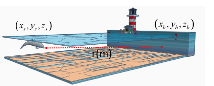
Figure 1: Model description

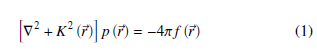
K(⃗r) is the medium wave number at radial frequency ω,∇ gradient operator, and p(⃗r) is the pressure. We can further simplify this equation to form the Helmholtz equation in two dimensions, as the sound speed and density depends only on depth z

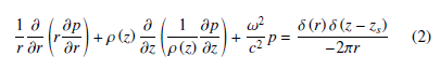
where r is the distance to the source, ρ is the medium density, c is the propagation speed, δ is the Dirac delta, and ω is angular velocity [6]. Using the separation of variables, we look for a depth-related pressure solution in the form of p(r,z) = ϕ(r)ψ(z), which will result in

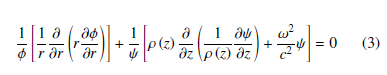
where ϕ is the volume displacement, and Ψ is the general modal depth function. Terms in square brackets of the equation (3) are functions of rand zrespectively. To satisfy the equation (3), each term should be equal to a constant [24]. Considering the Pekeris waveguide -where water is considered equal columns with varying speeds of propagation- We can drive the modal equation by considering the K_rm² as a separation constant [25].

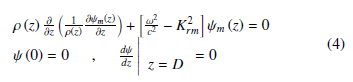
where ψ_m(z) is the particular modal function ψ(z) obtained with horizontal wave-number K_rm as separation constant. The boundary condition of the equation (4) considers each water column a pressure release surface (z = 0) and a perfectly rigid seabed at z = D (D < 100) which translates to no changes in the volume at surface and seabed resulting in dψ/dz = 0 [25].

Equation (4) is a classical Sturm-Liouville eigenvalue problem [24]. Applying the orthogonality of the modal Sturm-Liouville problem, we can write

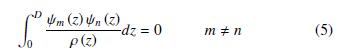
0Equation (3), the solutions of modal equations are arbitrary to multicaptive constants; therefore, we can further simplify the results using equation (5) as Z D ψ2m (z)

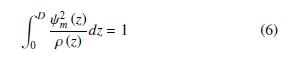
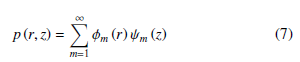
Moreover, modes transmit as a complete set, resulting in an arbitrary function as a sum of all normal modes, which will yield the pressure function as:

Substituting equation (7) in equation (2) provides :

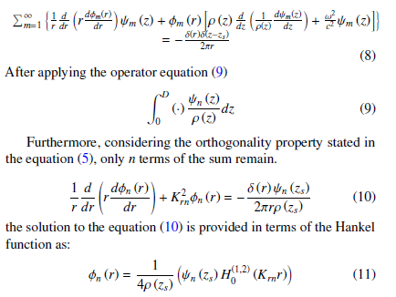
The signal’s energy radiates outwards, and therefore the solution will be H₀⁽¹⁾. Considering the radiation conditions, after substituting (11) in (7), we can derive the pressure equation based on the modal function as

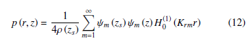
we can further simply equation (12) by using the asymptotic approximation to the Henkal’s function, yielding:

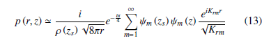
provides us with the pressure function, based solely on modal functions and depth.

2.2        Solution to Wave Equation

We must simplify the displacement equations further to perform channel modeling in simulation software. The non-homogeneous differential equation (1) can be solved using the Green’s function method and expanded as the displacement equation as [6, 23]

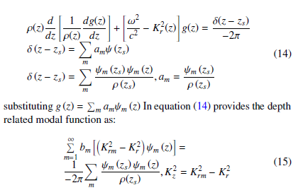
where K_rm, K_z, K_r are the angular, vertical and horizontal wavenumbers [26, 6]. applying Green’s solution to equation (15) would provide the general modal function:

 is the velocity of mode m at angular frequency ω.

2.3        Underwater Ambient Noise

Noise in a shallow underwater environment can be categorized into two main types, ambient noise caused by the channel characteristics and artificial noises created by external sources such as ships and marine life. Many studies consider the noise a simple added white noise; however, underwater ambient noise can be more accurately modeled as colored noise. The underwater channel’s behavior is best described as a low-pass filter. It can be modeled as a white noise sequence filtered using a Butterworth IIR low-pass filter with 30dB attenuation in stopband and normalized stopband frequency of 0.05 halfcyle/sample per sample ad 0.9 halfcyle/sample Respectively [27]. Figure 2 presents the signal and noise in the time domain with SNR=45dB.

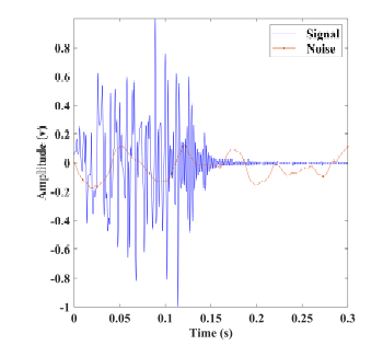
Figure 2: Signal (blue), Noise (red)

3. Modal Analysis based localization

In the previous section, we introduced the channel model and modal functions. In this section, we will derive the necessary equations for the localization of impulsive sound sources using modal functions. The modal-based localization methods are based on the dispersion of the natural frequencies as they propagate underwater.

3.1        Modal Dispersion

As stated earlier, modes travel at different speeds ( equation (17)), resulting in dispersion at the receiver. Let us consider the simulation scenario of Figure.1, where the Normal mode theory with ambient noise is used to model the channel. Considering an impulsive sound source at a depth of D_s=20m, 4000 meters away from the hydrophone, (ρ_(Seabed)=1000(Kg/m³), ρ_(Water)=1000(Kg/m³), c_(Seabed)=1500(m/s), c_(Water)=1600(m/s)), the propagated signal will have the time-frequency (TF) representation provided in Figure.3, which illustrates the dispersion caused by the difference in propagation speeds. One can employ the dispersion of modes to localize the sound source through modal analysis after filtering them.

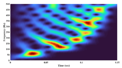
Figure 3: TF analysis, Modal dispersion , f_(Max)=600Hz

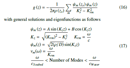
As the TF analysis graph illustrates, the dispersion curve’s frequencies overlap between the modes and render conventional filtering techniques inert. The overlapped frequencies are the product of the nonlinear phase characteristics in the equation (16).To address this issue, considering the pressure signal in the time domain as

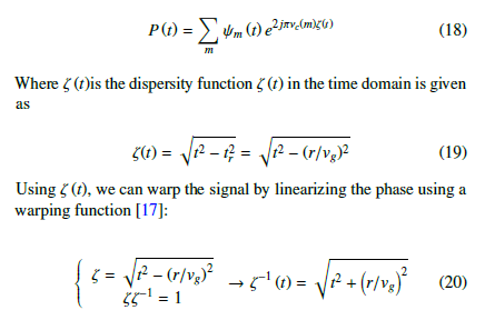
Applying the warping function ζ⁻¹ linearizes the phase. The TF graph of the linearized signal is presented in Figure 4.

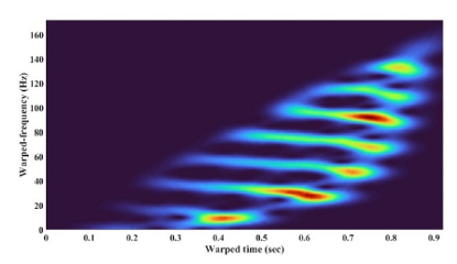
Figure 4: TF graph of warped signal

3.2        Localization Algorithm

Since the modal dispersion is directly related to the speed of propagation and distance, we can develop localization algorithms based on the TDOA concept. After filtering each of the dispersion curves; in an accurate channel model, the following expression will be true

Where τ_n is the dispersion curve. Measured τ_n can be obtained by warping and filtering each of the modals and by substituting the relationship between velocity and distance in the equation (17), the estimated τ_n can be obtained as:

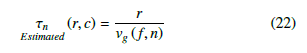
Where τ_n is the estimated dispersion curve for mode n transmitted over the range R with seabed sound speed c and group velocity υ_g (f,n). To localize the signal, we are looking for a range r that minimizes the statement (21). In other words

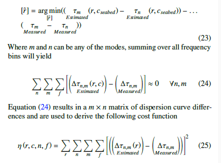
We employed a grid search algorithm to minimize the cost function η for values of r.

Algorithm 1 presents our proposed method where µ_r defines the localization step size in the search boundary [r_min,r_max] and ε is the accuracy of the estimated range. The Localization is performed in two steps; first, seabed and water parameters are defined based on the environment, and search boundaries for range and propagation speeds in seabed and sea are set. Next, the tensor of order 3, as shown in Figure 5, is formed to find the pairs of dispersion curves with the best performance (lowest value). Then, the cost function is formed only for the selected pairs of modes. Using a grid search algorithm, the location of the source can be estimated.

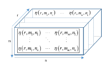
Figure 5: Cost function [ ]_r×m×n

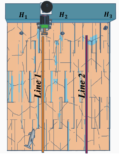
Figure 6: Model Description, multi hydrophone (H1,H2,H3)

Algorithm 1: Proposed localization Algorithm

Result: r

Initialization ˆr = (rmin : rmin + µr : rmax), ρwater,ρseabed;

Warp Input signal;

3.3        2D Localization

While most modal-based localization methods proposed by literature perform ranging, we propose a method for unsynchronized 2D localization with minimal hardware requirements. In the case of 2Dlocalization requirements, buoys (each with a single hydrophone) can transmit the received signals to a base station on shore or a vessel to be analyzed in a central processor. Although utilizing multiple hydrophones would require sensor synchronization in other methods, the proposed modal-based localization analyzes modes picked up by each hydrophone separately. Moreover, given the high-range localization capabilities, buoys can be placed far apart, reducing implementation costs. Figure 6 illustrates the model description for 2D localization, where lines Line1 and Line2 are assumed at coordinates [(x_H2 − x_H1)/2],[(x_H2 − x_H3)/2]. Given the distances of each buoy, each hydrophone’s average power of received modes is different. Hydrophones with the highest levels of received signal power are closest to the target. In the model description presented in Figure.6 ; P(B_H3) < P(B_H2) < P(B_H1) places the estimated latitude of the source Line1_H1H2 > x_s. Based on the estimated location of the source and three calculated ranges from each buoy, we can perform 2D triangulation and track an object without needing a synchronized sensor array.

4. Results and Discussions

This section includes numerical experiments to illustrate the proposed localization method and discusses the effects of ambient noise on the accuracy of the proposed algorithm. Modal analysis is suitable for processing underwater signals in long distances (r > 1000m) based on only one hydrophone without synchronization.

4.1        Simulated Sound

We consider an impulsive sound source is placed at Cartesian coordinates ( 4000,45,0) with a maximum frequency of 500 Hz. An Omni-directional hydrophone is located at (0,15,0). We assume the speed of propagation in the seabed c_b = 1600m/s, speed of propagation in water c_w=1500m/s, density in water ρ_w=1000kg/m³, and density in the seabed ρ_b=1500kg/m³. The performance is evaluated based on the cost function’s mean square error (MSE) and the estimated range’s Root Mean Square Error (RMSE). Moreover, the result of this study is compared with those of [17], which has used the same approach in localization.

Figure 7 (a),(b), and (c) illustrates the RMSE of the cost function for SNR=45dB,35dB, and 30dB values for each modal pair. As we can see, considering the low-pass filter nature of the ambient noise, the noise than others would more influence pairs of first and last modes. This is mainly due to both filter boundaries’ relatively low stop-band attenuation. This effect can compromise localization accuracy in low SNR environments. To address this issue, we proposed employing the cost-function MSE matrix of Figure 7, using the equation (25) to identify the best and most noise-resistant pairs of modes (lowest values), resulting in the lowest MSE. After identifying the best modal pairs (2 pairs in this study), we can find the estimated location of the acoustic sound source through the equation (23).

Figures 7 (a), (b), and (c) depict the Root Mean Square Error (RMSE) of the cost function for SNR values of 45dB, 35dB, and 30dB, respectively, for each pair of modes. It can be observed that, due to the low-pass filter characteristics of ambient noise, certain modal pairs are more influenced by noise compared to others. This effect is particularly prominent in the first and last mode pairs, primarily because of the relatively low stop-band attenuation at the boundaries of the filter. In low SNR environments, this influence can significantly compromise localization accuracy. Furthermore, Figure 7 demonstrates that the choice of modal pairs significantly impacts the error levels, as different pairs yield varying levels of error. The study presented in [17] solely employs modal pairs with sequential wavenumbers numbers, disregarding the performance of different pairs. To address this issue, we propose utilizing the MSE matrix of Figure 33 as the cost function, employing equation (25) to identify the most noise-resistant and optimal pairs of modes (with the lowest values). This selection process leads to lower MSE and enables us to determine the estimated location of the acoustic sound source using equation (23).

Figure 8a showcases the Root Mean Square Error (RMSE) of our proposed cost function for range estimation at different SNR levels, and it compares these results with the localization outcomes presented in [17]. Figures 8a and 8b clearly demonstrate that our proposed method exhibits superior performance in both low and high SNR environments. This improvement can be attributed to the fact that the localization method employed in [17] does not incorporate mode pair evaluation or selection. Instead, they utilize pairs of modes with consecutive mode numbers in their localization algorithm. However, as indicated in Figure 7, sequential mode numbers do not necessarily yield better localization results. By performing mode evaluation and selection, as shown in Figures 8a and 8b, the localization algorithm becomes more resilient to high levels of noise and achieves greater accuracy.

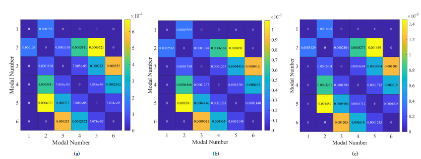
Figure 7: Cost function MSE for (a)SNR:45dB, (b)35dB, (c)30dB

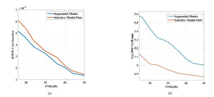
Figure 8: Time Frequency Representation (TFR) of (a) Cost Function RMSE (b) Log(RMSE) of estimated range for: 28dB < SNR < 45dB

4.2        Recorded North Atlantic Whale and Explosion Sound Localization

In this section, we conduct a comprehensive evaluation of our proposed selective weighted algorithm using two distinct sound sources: the sound of a North Atlantic Right Whale and an explosion sound. Figure 9 depicts the time series and time-frequency (TF) analysis of these signals transmitted over different distances: 4.5 Km (z=20m) for the explosion sound and 8.7 Km (z=66m) for the whale sound. The TF analysis reveals that the noisy signal representing the explosion has a maximum frequency of 450 Hz, while the whale sound exhibits a lower maximum frequency of approximately 350 Hz. Furthermore, it is evident that certain modes are more susceptible to interference, highlighting the significance of modal selection and weighting functions in our approach.

We proceeded to localize the two signals and compared our results with our previous work and other existing methods. Table 1 presents the localization outcomes, demonstrating notable improvements compared to other proposed methods. Our Selective-modal based localization (SMP) approach achieved an error rate of 2.6% for both the recorded explosion sound and whale sound, while the Sequential Pair-Mode Analysis (SM) method yielded error rates of 3.11% and 6.2% for the respective signals. The superior performance of our proposed SMP method can be attributed to employing a larger number of dispersion curves (as opposed to only six sequential dispersion curves in SM) and performing initial modal selection.

Despite these improvements, it is important to note, as indicated in the TF analysis of Figure 9 and discussed in Section 3, that noise and channel effects vary across different modes. Consequently, each mode exhibits different weights and importance in the localization process, a consideration that is addressed in our approach.

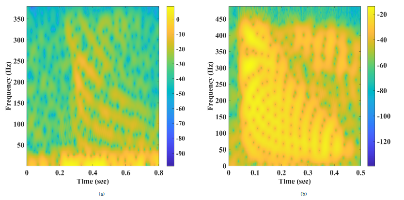
Figure 9: TF analysis: (a) North Atlantic Whale (b) Underwater Explosion

4.3        2D Localization

In this section, we conduct a comparative analysis of the 2D tracking performance of our localization algorithm in relation to other methods. Using the model description outlined in Figure 6, we employed a simulated non-stationary impulsive sound source that closely resembles the characteristics of a traveling whale following a sinusoidal path along the (x,y) axis.

Our 2D localization approach involves estimating the range of the sound source to each buoy, followed by triangulation based on the approximate direction of arrival and the intersection point of circles with a radius of r_h. The localization results for both the Sequential modes (SM) and our proposed Selective-modal based localization (SMP) are depicted in Figure 9, along with the true location of the sound source. It is evident from the results that SMP exhibits a closer adherence to the true range line compared to SM. This improved performance can be attributed to the modal selection function we introduced in this paper, which enables more accurate localization of the sound source.

5. Conclusion

In this study, we presented a passive impulsive sound source localization approach specifically designed for shallow underwater environments. Our method utilized the normal mode channel model and ambient noise to achieve accurate localization. A key contribution of this paper is the introduction of a localization scheme that incorporates modal pair selection, enabling enhanced noise resistance and improved accuracy.

Additionally, we proposed a 2D localization technique suitable for unsynchronized hydrophones, which aligns with the requirements of existing remote monitoring systems. To evaluate the performance of our algorithm, we conducted extensive analyses under various signal-to-noise ratio (SNR) conditions, comparing its noise resistance capabilities with other methods.

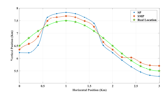
Figure 10: 2D localization and tracking of an impulsive sound source

Furthermore, we validated our algorithm by testing it with actual recorded whale and explosion sounds. The results demonstrated its effectiveness in accurately tracking impulsive sound sources in a 2D space. Overall, our proposed approach showcases advancements in impulsive sound source localization and offers notable improvements over existing techniques.

1. F. Talebpour, S. Mozaffari, M. Saif, S. Alirezaee, “Multi-Modal Signal Analysis for Underwater Acoustic Sound Processing,” in 2022 IEEE Canadian Confer- ence on Electrical and Computer Engineering (CCECE), 300–305, IEEE.
2. X. Su, I. Ullah, X. Liu, D. Choi, “A Review of Underwater Localization Tech- niques, Algorithms, and Challenges,” Journal of Sensors, 2020, 1–24, 2020, doi:10.1155/2020/6403161.
3. R. Vaccaro, “The past, present, and the future of underwater acoustic signal processing,” IEEE signal processing magezine, 15(4), 21–51, 1998.
4. V. Kavoosi, M. J. Dehghani, R. Javidan, “Underwater Acoustic Source Posi- tioning by Isotropic and Vector Hydrophone Combination,” Journal of Sound and Vibration, 501, 116031, 2021, doi:10.1016/j.jsv.2021.116031.
5. K. F. Bou-Hamdan, A. H. Abbas, “Utilizing ultrasonic waves in the investi- gation of contact stresses, areas, and embedment of spheres in manufactured materials replicating proppants and brittle rocks,” Arabian Journal for Science and Engineering, 47(9), 11635–11650, 2022.
6. D. A. Abraham, Underwater Acoustic Signal Processing: Modeling, Detection, and Estimation, Springer, 2019.
7. D. Neupane, J. Seok, “A Review on Deep Learning-Based Approaches for Automatic Sonar Target Recognition,” Electronics, 9(11), 1972, 2020, doi: 10.3390/electronics9111972.
8. W. A. Kuperman, J. F. Lynch, “Shallow-Water Acoustics,” Physics Today, 57(10), 55–61, 2004, doi:10.1063/1.1825269.
9. S. M. Wiggins, M. A. McDonald, L. Munger, S. E. Moore, J. A. Hildebrand, “Waveguide propagation allows range estimates for North Pacific right whales in the Bering Sea,” Canadian acoustics, 32, 146–154, 2004.
10. M. Sanguineti, J. Alessi, M. Brunoldi, G. Cannarile, O. Cavalleri, R. Cerruti, N. Falzoi, F. Gaberscek, C. Gili, G. Gnone, D. Grosso, C. Guidi, A. Mandich, C. Melchiorre, A. Pesce, M. Petrillo, M. G. Taiuti, B. Valettini, G. Viano, “An automated passive acoustic monitoring system for real time sperm whale (Physeter macrocephalus) threat prevention in the Mediterranean Sea,” Applied Acoustics, 172, 107650, 2021, doi:10.1016/j.apacoust.2020.107650.
11. L. An, L. Chen, “A real-time array calibration method for underwater acoustic flexible sensor array,” Applied Acoustics, 97, 54–64, 2015, doi: 10.1016/j.apacoust.2015.04.008.
12. F. B. Jensen, W. A. Kuperman, M. B. Porter, H. Schmidt, A. Tolstoy, Computa- tional ocean acoustics, volume 794, Springer, 2011.
13. S. Khazaie, X. Wang, P. Sagaut, “Localization of random acoustic sources in an inhomogeneous medium,” Journal of Sound and Vibration, 384, 75–93, 2016, doi:10.1016/j.jsv.2016.08.004.
14. G. Wang, S. Cai, Y. Li, M. Jin, “Second-Order Cone Relaxation for TOA- Based Source Localization With Unknown Start Transmission Time,” IEEE Transactions on Vehicular Technology, 63(6), 2973–2977, 2014, doi:10.1109/ tvt.2013.2294452.
15. Y. Zou, H. Liu, Q. Wan, “An Iterative Method for Moving Target Localization Using TDOA and FDOA Measurements,” IEEE Access, 6, 2746–2754, 2018, doi:10.1109/access.2017.2785182.
16. P. Wu, S. Su, Z. Zuo, X. Guo, B. Sun, X. Wen, “Time Difference of Arrival (TDoA) Localization Combining Weighted Least Squares and Firefly Algo- rithm,” Sensors (Basel), 19(11), 2554, 2019, doi:10.3390/s19112554.
17. J. Bonnel, A. Thode, D. Wright, R. Chapman, “Nonlinear time-warping made simple: A step-by-step tutorial on underwater acoustic modal sepa- ration with a single hydrophone,” J Acoust Soc Am, 147(3), 1897, 2020, doi:10.1121/10.0000937.
18. E. Xu, Z. Ding, S. Dasgupta, “Source Localization in Wireless Sensor Net- works From Signal Time-of-Arrival Measurements,” IEEE Transactions on Signal Processing, 59(6), 2887–2897, 2011, doi:10.1109/tsp.2011.2116012.
19. R. Diamant, L. Lampe, “Underwater Localization with Time-Synchronization and Propagation Speed Uncertainties,” IEEE Transactions on Mobile Comput- ing, 12(7), 1257–1269, 2013, doi:10.1109/tmc.2012.100.
20. A. Thode, J. Bonnel, M. Thieury, A. Fagan, C. M. Verlinden, D. Wright, J. Crance, C. L. Berchok, “Using nonlinear time warping to estimate North Pacific right whale calling depths and propagation environment in the Bering Sea,” Journal of the Acoustical Society of America, 142(4), 2711–2712, 2017.
21. H. Jia, X. Li, “Underwater reverberation suppression based on non-negative matrix factorisation,” Journal of Sound and Vibration, 506, 116166, 2021, doi:10.1016/j.jsv.2021.116166.
22. Y. Tian, M. Liu, S. Zhang, T. Zhou, “Underwater multi-target passive detec- tion based on transient signals using adaptive empirical mode decomposition,” Applied Acoustics, 190, 108641, 2022.
23. C. T. Tindle, A. Stamp, K. Guthrie, “Virtual modes and the surface bound- ary condition in underwater acoustics,” Journal of Sound Vibration, 49(2), 231–240, 1976.
24. E. Costa, L. Godinho, W. Mansur, Peters, “Prediction of Acoustic Wave Propa- gation in Underwater Step Problems via the Method of Fundamental Solutions,”
    European Acoustics Association, 2016.
25. C. L. Pekeris, Theory of propagation of explosive sound in shallow water, Geological Society of America, 1948.
26. R. P. Hodges, Underwater acoustics: Analysis, design and performance of sonar, John Wiley and Sons, 2011.
27. Q. Yang, K. Yang, “Seasonal comparison of underwater ambient noise observed in the deep area of the South China Sea,” Applied Acoustics, 172, 107672, 2021, doi:10.1016/j.apacoust.2020.107672.
28. C. Gervaise, S. Vallez, Y. Stephan, Y. Simard, “Robust 2d localization of low-frequency calls in shallow waters using modal propagation modelling,” Canadian Acoustics, 36(1), 153–159, 2008.
29. F. Desharnais, M. Coˆte´, C. J. Calnan, G. R. Ebbeson, D. J. Thomson, N. E. Collison, C. A. Gillard, “Right whale localisation using a downhill simplex inversion scheme,” Canadian Acoustics, 32(2), 137–145, 2004.
30. M. H. Laurinolli, A. E. Hay, “Localisation of right whale sounds in the work- shop Bay of Fundy dataset by spectrogram cross-correlation and hyperbolic fixing,” Canadian Acoustics, 32(2), 132–136, 2004.

(Click Here)