1. Introduction

There are many solutions for reconstructing 3D structure based on optical flow vectors of 2D images taken by camera(s) mounted on mobile robot. However, the proposed solutions are not be feasible if the optical flow image contains noise vectors. One of the approaches to remove noise in optical flow vectors introduced at the conference ICECCME-2022 [1] makes it possible to study optical flow images on unstable light conditions based on an optical flow noise filter with dynamic thresholds computed by relatively comparing between the average magnitude value of optical flow vectors and an outlier magnitude value. After removing noise vectors, optical flow imaging can be used for mobile robots to observe the working environment and perform complex tasks. Derived from noise-free optical flow images, this article is the next extension of [1] in aspect of experimental simulation of obstacle detection from the noise-free optical flow images to help mobile robots move safely in a simulated indoor office environment.

Over the past decades, mobile robots have been widely used in many production areas such as industry [2] and agriculture [3], in service activities such as search and rescue [4] and in offices [5]. Mobile robots have proven to be effective in supporting humans through their ability to move flexibly and safely in various ways such as by wheels [6], crawlers [7], omnidirectional wheels [8]. Many kinds of sensors such as infrared [9], ultra-sonic [10] and laser [11] have been applied to help mobile robots recognize the surrounding context and make corresponding decisions according to the set requirements. Among the studies of the sensor-based recognition on mobile robots, image-based recognition solutions have been studied a lot thanks to their ability to recognize many objects with different shapes, sizes and distances [12].

Based on the acquired images, the robot performs 2D or 3D scene reconstruction to identify objects to distinguish between a target (to approach) and an obstacle (to avoid). However, image processing often has to deal with the difficult problems of processing time and noise in captured images [13]. The optical flow vector-based identification solution is researched on the idea of biomimetic mimicry of bees in observing, acquiring and processing dynamic image information [14]. Technically, classical techniques of optical flow recognition usually use the method of comparing the difference in vector density of the left half with that of the right half to determine the direction of the obstacle [15].

In this study, the obstacle detection solution based on optical flow images filtered out noise vectors will be tested on a simulated environment with some situations related to different density of obstacles. The movement trajectory of the robot is automatically recorded to analyze and evaluate the safe movement when passing through the areas arranged many obstacles randomly.

The next content is organized as follows: Firstly, the optical flow processing is introduced. Then, the solution of locating obstacle from noise-free optical flow images is analyzed.  After that, the simulation of optical flow-based mobile robot moving and avoiding obstacles in a simulated office is depicted and analyzed. Finally, the conclusion are drawn.

2. Optical flow processing

The processing of real optical flow vectors is shown in Figure 1a and that of simulation noise-free optical flow vectors is illustrated in Figure 1b. The multi-layer segmentation of the optical flow vectors depicted in Figure 1 can be explained as the following schedule:

In the first processing stage, the optical flow image is divided into four equal parts Q₁, Q₂, Q₃ and Q₄. Mathematically, the average magnitude matrix of optical flow vectors in the first processing stage is formulated as follows:

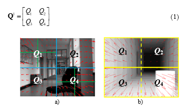
Figure 1: Segmentation of real (a) and simualtion (b) noise-free optical flow images.

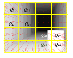
Figure 2: Segmentation in the second processing stage.

Figure 2 illustrates the second stage of multi-layer segmentation of optical flow vectors. In this stage, the four first processing parts are divided into four smaller parts Q_1i, Q_2i, Q_3i and Q_4i, where i = 1…4. The average intensity matrix of the optical flow vectors in the second processing stage has the following form:

By the similar way, in the n^th processing stage, the four parts of the (n-1)^th processing stage are divided into four smaller parts of the deeper layer of the processing, that means  Q¹, Q², … and Qⁿ  are matrices of average magnitude of optical flow vectors in processing stage 1, 2,… and n, respectively.

3. Locating obstacle from noise-free optical flow images

To detect obstacle position during robot movement, various depth-based recognition methods [12] and [16] are implemented by processing images captured by a single camera mounted on the mobile robot. Similarly, optical flow vector images are analysed after multi-layer segmentation to locate the obstruction areas and obtain depth information through qualitative calculations. In other words, the basic principle of determining the location of obstacles is to identify a part of the image having the average Q_i bigger than the others in the magnitude matrix of optical flow vectors.

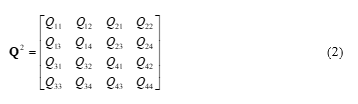
Figure 3 illustrates the way for locating the obstacle based on the multi-layer segmentation of optical flow vectors. It is easy to see in Figure 3a that in the first processing stage, part Q₄ has the biggest magnitude due to covering the obstacle. In the second processing stage shown in Figure 3b, parts Q₄₂ and Q₄₄ have the biggest magnitudes because the obstacle fills all these parts compared to half filling in parts Q₄₁ and Q₄₂.

Figure 3: Locating obstacle from optical flow image: a) layer-1; b) layer-2.

As shown in Figure 4, an optical flow vector  contains two components projected onto axes OU and OV as follows:

where  and   are unit vectors, u_ij and v_ij are amplitudes of a vector  projected on axes OU and OV, respectively.

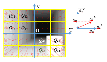
Figure 4: Projecting an optical flow vector  onto axes OU and OV

Let consider Q₄₄ containing 16 optical flow vectors arranged in four rows and four columns by the following matrixes:

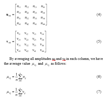
where n is number of components at column j. As the illustration in Figure  4, n = 4 and j = 1…4.

From equation (4) and (6), let compare the average value  of all u_ij in one column and replace the biggest average by 1, we have the matrix of obstacle direction as follows:

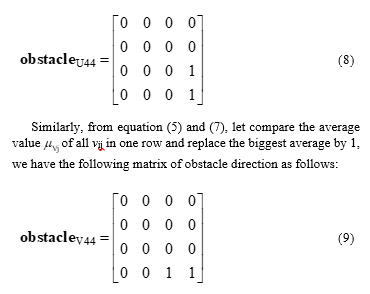
Based on the equation (8) and (9), the mobile robot can locate the most dangerous area in the noise-free optical flow image.

4. Simulation

4.1.  Simulation setup

The mobile robot control system with a camera is simulated on the Matlab program and organized into functional modules as illustrated in Figure  5. The two coordinate systems including the mobile robot’s coordinate system (body frame) related to the motion parameters of the simulated mobile robot and the office’s coordinate system (inertial frame) related to the office environment are shown in Figure  6.

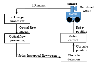
Figure 5: Simulated control system of mobile robot

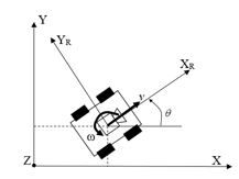
Figure 6: Two coordinate systems and motion parameters of mobile robot

The motion in the simulated mobile robot’s coordinate system (OXYZ)_R can be defined from the office’s coordinate system (OXYZ) as follows:

where

– v, ω, and θ are the linear velocity, angular velocity, and rotational angle of the robot’s coordinate system related to the office’s coordinate system, respectively.

– , , and  are the linear velocities and the rotational angular velocity, respectively because the variable x, y and θ are positions and rotational angle of the robot , respectively.

– R_z is the rotation matrix on the Z-axis.

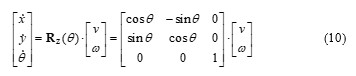
The simulated robot has a width of 50 cm and a length of 60 cm. The office is simulated as shown in Figure  7 to test the robot’s ability to move through the recorded camera images. The top view of the simulated office in Figure 7a shows that there are four rooms in the central area and some doors connecting the rooms to the corridor surrounding the office. The side view of the office in Figure 7b provides door (entrance) and ceiling height information. The width of the entrance is 130 cm and the height of the ceiling is 350 cm. A typical camera image is extracted to visualize the robot’s view of the work area as the illustration in Figure 7c.

The main objective of the experiments is to test robot’s ability to avoid obstacles randomly arranged along the road in different situations based on the result of noise-free optical flow recognition.

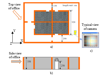
Figure 7: Simulated office for testing obstcle avoidance of mobile robot

4.2.  Simulation results

The simulation is performed by the Matlab program with the computer speed 3.40GHz of Intel(R) Pentium(R) 4 CPU and the image processing is carried out by the GPU NVIDIA GeForce GTX 260 1.24GHz with segment size 32 x 32 pixels.

1. a) Simulated environment image without obstacles

Before testing the robot’s ability of obstacle detection, we should review the typical contexts without obstacle in the simulated office situations related to walls, corners, doors and corridors.

Optical flow images are shown in Figure  8 when the robot copes with the walls: the straight view of the camera to a wall (Figure  8a) and the slanted view of the camera to the wall (Figure  8b).

Figure 8: Optical flow images of wall: a) straight view, b) slanted view

Optical flow images are depicted in Figure  9 as the robot approaches the corners of the office: straight view of the corner center (Figure  9a) and slanted view of the corner center (Figure  9b).

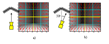
Figure 9: Optical flow images of corner: a) straight view, b) slanted view

Optical flow images are illustrated in Figure  10 as the robot approaches the doors of the office: straight view of the door center (Figure  10a) and slanted view of the door center (Figure  10b).

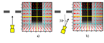
Figure 10: Optical flow images of door: a) straight view, b) slanted view

Optical flow images are sketched in Figure  11 during the robot following the corridors of the office without any obstacle: straight view of the corridor (Figure  11a) and slanted view of the corridor (Figure  11b).

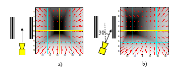
Figure 11: Optical flow images of corridor: a) straight view, b) slanted view

The statistical data of optical flow images are shown by colorful 3D histograms in Figure  12 for different distances (right horizontal axis) including near (blue), middle (yellow) and distal (red) for different objects including walls (A1), corners (A2), doors (A3) and corridors (A4) in 4 depth stages of optical flow vector processing (vertical axis) to evaluate tilt angles between the camera and the observed object by measuring the ratio of the mean value between the left optical quadrant and the right optical quadrant (nearest horizontal axis).

It is easy to see that the optical flow vectors in these situations are distributed differently between images despite the absence of obstructions. However, in the cases of close distances to the objects, the robot still has to avoid the nearest object as if avoiding an obstacle. Based on the ratio between the left parts and the right part, the principle for avoiding obstacle is that the robot travels to the direction containing the smaller average value between left and right optical flow parts.

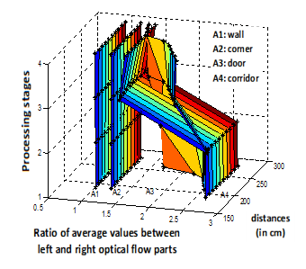
Figure 12: Ratio of average values between left and right optical flow parts.

1. b) Simulation test with low obstacle density

In the first test, the robot moved along a corridor containing several obstacles randomly arranged along the path illustrated in Figure 13. On the moving trajectory, the robot has to detect obstacles through the noise-free optical flow vectors.

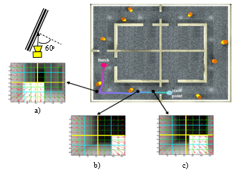
Figure 13: Robot avoids single obstacles

The robot movement is automatically recorded and depicted by a colorful truth-ground line. Along this line, several images are extracted to demonstrate that the robot has moved from the right to the left of the corridor and avoided a close front left obstacle (Figure  13a), a close right obstacle (Figure  13b), and a far front right obstacle (Figure  13c). The line with the three extracted optical flow images show the obstacle positions detected from the optical flow vectors and the robot succeeded in moving safely by avoiding the two detected obstacles.

In the second test, the robot travelled along a different part of the corridor. It has to avoid not only a single obstacle but also a pair of obstacles on the corridor. The robot movement trajectory is automatically recorded by a colorful truth-ground line as shown in Figure  14. Along the line, several images are taken out to prove that the robot has moved from the right to the left of the corridor. The robot avoided a close front obstacle (Figure  14a), a pair of obstacles (Figure  14b) in far distance, and a pair of obstacle and wall (Figure  14c).

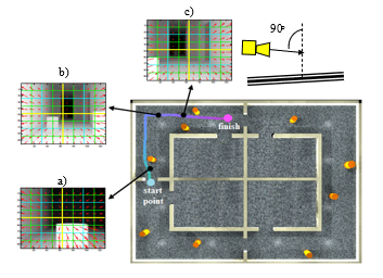
Figure 14: Robot avoids a pair of obstacles

The successful movements of the robot in the two first tests verify the robot’s ability of obstacle detection based on the optical flow vectors taken from the simulated images.

1. c) Simulation test with high obstacle density

In the third test, the robot performed the more difficult task of safe movement through the corridor containing much more obstacles randomly arranged in a cramped area.

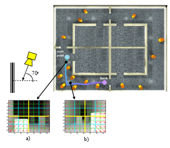
Figure 15: Robot avoids many obstacles in a cramped area

Technically, the solution of dividing the optical flow vector into multiple layers allows the robot system to compare the average magnitude of a part with other parts in the same layer. That means it can detect multiple obstacles at the same time and estimate the distance through the magnitude of the average vector. As a result, the robot can choose the appropriate (possibly suboptimal) movement direction to avoid obstacles.

The moving trajectory of the robot through the narrow area with many obstacles is automatically recorded by the colored line illustrated in Figure  15. Along this line, two images are extracted to represent the movement trajectory of the mobile robot after avoiding the closest obstacle on the left (Figure  15a), passing the area with high obstacle density, and avoiding another close obstacle on the right (Figure  15b) before leaving the danger area successfully.

5. Discussion and Conclusion

The above simulation results not only show the stability of optical flow perception in different situations, but also show that the obstacle position detection based on optical flow is independent of the robot’s speed. Thanks to the simple calculation method based on the average vector comparison method, the robot does not need large memory to store complex database of obstacle characteristics such as shape and size.

In other words, the simulation results of obstacle detection based on optical flow free-noise images for mobile robot demonstrate that the recognition of dangerous area in the optical flow image is able to perform through the multi-layer processing of optical flow vectors in to many equal parts. By simply comparing the average magnitude values of the divided parts, the mobile robot can figure out obstacle positions to guide the robot follow a suitable safe way.

The limitation of the simulation results is that the mobile robot copes with static obstacles, but not dynamic obstacles. This indicates that in the next phase, the research team need to build an actual mobile robot to test in real environments with dynamic obstacles to more accurately assess the stability of the optical flow-based recognition method.

Furthermore, in the future the real tests will be performed in a complex indoor environment with unstable lighting conditions to estimate the ability of optical flow-based recognition.

Conflict of Interest

The author declares no conflict of interest.

1. N. Anh Mai, “Multi-layer segmentation solution to filter the noise of optical flow vectors to assist robots in object recognition inside buildings,” International Conference on Electrical, Computer, Communications and Mechatronics Engineering, ICECCME 2022, (November), 16–18, 2022, doi:10.1109/ICECCME55909.2022.9988355.
2. A. Markis, M. Papa, D. Kaselautzke, M. Rathmair, V. Sattinger, M. Brandstotter, “Safety of Mobile Robot Systems in Industrial Applications,” Proceedings of the ARW & OAGM Workshop 2019, 26–31, 2019, doi:10.3217/978-3-85125-663-5-04.
3. S.S.H. Hajjaj, K.S.M. Sahari, “Review of research in the area of agriculture mobile robots,” Lecture Notes in Electrical Engineering, 291 LNEE(January 2018), 107–118, 2014, doi:10.1007/978-981-4585-42-2_13.
4. N. Ruangpayoongsak, H. Roth, J. Chudoba, “Mobile robots for search and rescue,” Proceedings of the 2005 IEEE International Workshop on Safety, Security and Rescue Robotics, 2005(July), 212–217, 2005, doi:10.1109/SSRR.2005.1501265.
5. W. Chung, G. Kim, M. Kim, C. Lee, “Integrated Navigation of the Mobile Service Robot in Office Environments,” International Conference on Control, Automation, and Systems (ICCAS), 2033–2038, 2003.
6. M. Trojnacki, P. Dąbek, “Mechanical properties of modern wheeled mobile robots,” Journal of Automation, Mobile Robotics and Intelligent Systems, 13(3), 3–13, 2019, doi:10.14313/JAMRIS/3-2019/21.
7. A. Dobrokvashina, R. Lavrenov, E. Magid, Y. Bai, M. Svinin, R. Meshcheryakov, “Servosila Engineer Crawler Robot Modelling in Webots Simulator,” International Journal of Mechanical Engineering and Robotics Research, 11(6), 417–421, 2022, doi:10.18178/ijmerr.11.6.417-421.
8. K. Kanjanawanishkul, “Omnidirectional wheeled mobile robots: Wheel types and practical applications,” International Journal of Advanced Mechatronic Systems, 6(6), 289–302, 2015, doi:10.1504/IJAMECHS.2015.074788.
9. M. Al-Mallah, M. Ali, M. Al-Khawaldeh, “Obstacles Avoidance for Mobile Robot Using Type-2 Fuzzy Logic Controller,” Robotics, 11(6), 2022, doi:10.3390/robotics11060130.
10. S. Adarsh, S.M. Kaleemuddin, D. Bose, K.I. Ramachandran, “Performance comparison of Infrared and Ultrasonic sensors for obstacles of different materials in vehicle/ robot navigation applications,” IOP Conference Series: Materials Science and Engineering, 149(1), 2016, doi:10.1088/1757-899X/149/1/012141.
11. J. Cai, T. Matsumaru, “Human detecting and following mobile robot using a laser range sensor,” Journal of Robotics and Mechatronics, 26(6), 718–734, 2014, doi:10.20965/jrm.2014.p0718.
12. T.A.Q. Tawiah, “A review of algorithms and techniques for image-based recognition and inference in mobile robotic systems,” International Journal of Advanced Robotic Systems, 17(6), 1–25, 2020, doi:10.1177/1729881420972278.
13. Y. Zhu, C. Huang, “An Improved Median Filtering Algorithm for Image Noise Reduction,” Physics Procedia, 25, 609–616, 2012, doi:10.1016/j.phpro.2012.03.133.
14. M. Egelhaaf, “Optic flow based spatial vision in insects,” Journal of Comparative Physiology A: Neuroethology, Sensory, Neural, and Behavioral Physiology, (0123456789), 2023, doi:10.1007/s00359-022-01610-w.
15. Y. Zhang, R. Huang, W. Nörenberg, A.B. Arrenberg, “A robust receptive field code for optic flow detection and decomposition during self-motion,” Current Biology, 32(11), 2505-2516.e8, 2022, doi:10.1016/j.cub.2022.04.048.
16. Z. El Kadmiri, O. El Kadmiri, L. Masmoudi, “Depth estimation for mobile robot using single omnidirectional camera system,” Journal of Theoretical and Applied Information Technology, 44(1), 29–34, 2012.

(Click Here)