1. Introduction

This paper is an extension of work originally presented in CICS2021 [1]. After the presentation at the conference CICS2021, we have done more researches on this issue and more interesting empirical results are obtained and updated in this extension version.

In the past decades, many approaches have been developed to tackle a time-varying time series. The main idea is how to separate the whole data set(interval) into several subsets(subintervals) with different statistical characteristics.

One of the methodologies is to detect change point or structural change in data [2]–[9]. One is to track the time-varying series using a Particle Filter [10], [11]. But, in this study, we propose to apply the Markov Regime Switching Analysis (MRSA) models to the time-varying data. The reason is that a time-varying series canbe efficiently and appropriately split into several subintervals with different statistical characteristics(or different state-specific regimes) by using the MRSA models. Namely, the dynamics of these subintervals can be well captured by MRSA [12]–[21].

And in many cases the regime changes are corresponding to the change points. Regimes indicate the situations of the infected cases, or the specific-state subintervals(market states). GARCH(Generalised Autoregressive heteroscedasticity) model [22], [23]. Since GARCH model can help us get different and consecutive subintervals based on the conditional heteroscedasticity and has been utilized ranging from finance to psychology [24]–[27]. We fit the stock returns of DAX Index and the growth rates of COVID-19 to GARCH models to get their volatilities. And then apply MRSA to the volatilities, to investigate and assess the impact of the pandemic on the German stock market [1], [12]–[21].

Focusing upon the changes of DAX Index is that Germany is the industry leader country in the Europe Union(EU), it is important to know what impact had on the German stock market during the COVID-19 pandemic. Knowing what may happen during a pandemic, we can predict and do more better while dealing with another pandemic in the future.

The remainder of this paper is organized as follows. Section 2 shows an overview of our proposed Markov Regime Switching Analysis(MRSA). Section 3 explains the data sets we use in this study. Section 4 summarizes the outbreak situations in Germany. Section 5 presents our empirical results in situation analysis of the disease outbreak, and its impact on the market, by using the MRSA models. Section 6 displays the MRSA results by using the volatilities obtained by the GARCH model fittings. Section 7 gives concluding remarks.

2. An Overview of Markov Regime Switching Analysis

We here just give an overview of Markov Regime Switching Analysis before we present the results of our empirical analyses below [12]–[21]. Usually MRSA is utilized to depict the dynamics of a time series by using regime states. Regime states describe the different segments of a time series in different states. The common example of regime states is of two different states, denoted as s_t, either s_t = 0 or s_t = 1, presenting two different regimes.

A common MRSA model is to do regression assuming different regime states existing in the data. The advantage of this method is that one can expose the varieties around the means. Such as,

where s_t = 0 or 1 means that data y_t have two different mean levels in different segments, where ϵ_t follows a Gaussian process with mean zero and variance σ². State zero (s_t=0) corresponds to Regime 1, and verse vice.

Another usage of MRSA is to build an Markov regime switching autoregressive Model. A generalised presentation of the model can be described as follows, assuming the AR model with order p, namely,

where x_t is called as exogenous variable. The transition probabilities are usually defined as a first order Markov chain. Thus, a transition probability matrix P with n states can be represented as follows.

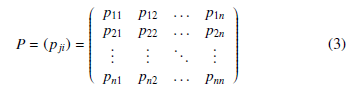
where i, j = 1,2,…n, with ^Pn_j=1 p_ji = 1, and p_ji is the probability of transitioning from regime i to regime j.

While, a simplified case of (2) is that a Markov regime switching autoregressive model without an exogenous variable.

The following model shows the time-varying data y_t follows two different AR(1) equations with different parameters, for example.

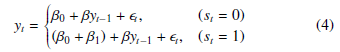
What (1)-(4) mean is that the time-varying observations fluctuate when state or regime shifts from one to another.

The estimation of parameters of regime-switching models is implemented by maximizing the likelihood function.

3. Data Description

In this study, we use the following two data sets.

• DAX(daily), which is known as the GER40 as well, comprised of 40 German companies traded on the Frankfurt Exchange. We obtained the data from Yahoo(https://de.finance.yahoo.com). The period of the data set is ranged from Jan, 2020 to Jul, 2021.
• The newly infected cases of COVID-19(daily). We obtained the data from WHO’s Website, in the same period.

These two data sets are open to the public on above-mentioned websites, and can be downloaded freely, at any time.

4. Situations of COVID-19 Outbreak

Germany is the industry leader in the Europe Union(EU), and it is important to investigate how the German stock market was impacted from the pandemic. We thus focus upon the situations in Germany.

In Germany, the ups and downs of the newly confirmed number(daily) are shown in Figure 1, duration from January 22, 2020 to July 30, 2021.

All Deseasoned Series

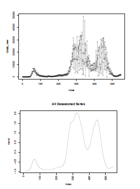
Figure 1: Daily newly confirmed number(left) and its trend(right)

It shows the newly confirmed number(daily) fluctuated with the lapse of time. The left small peak appeared when fewer cases were confirmed. However, gradually the newly confirmed number rose from zero level up to a big peak, and then decayed to its half level around. Sooner, the third peak appeared when the newly confirmed number surged once more. One may be interested in identifying change points, we had successfully identified the change points in this time series based upon a Bayesian approach[8], [9].

With the spread of infection of COVID-19 in Europe, lockdown policy had been employed in many countries, since the newly confirmed cases were growing up and up. The government enforced lockdown in Nov, 2020, and it had not been lifted until Jun, 2021, about 8 months long. Besides, mask-wearing, social distancing, staying home and other public health measures had been also implemented, these measures had shown their effects on reducing newly infected cases.

5. Empirical Research

We then carry out some empirical analyses by using the abovementioned two data sets.

5.1        Markov Switching Regression Analysis

Firstly, the Markov regime switching regression model is applied to the data. Table 1 shows the estimated results.

Table 1: Estimated results

Intercept	Regime 1	Regime 2
Estimate	12889	844.336
Std. Error	557	43
t value	23	19
Pr(> |t|)	2.2e-16***	2.2e-16***
AIC	10178.62
Likelihood	-5087.31

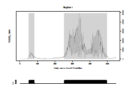
Figure 2: Regime 1 is represented in gray

Figure 2 shows the estimated areas of Regime 1 in gray. Seen from the figure, the peaks of daily infected number are identified as Regime 1 in gray, and verse vice.

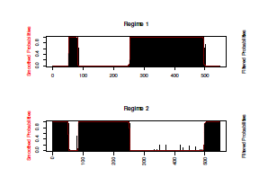
Figure 3: Plots of estimated probabilities of Regime 1 and 2

Figure 3 displays the estimated transition probabilities of Regime 1 and 2.

The corresponding transition probabilities are estimated and shown in Table 2. While, the corresponding confidence intervals(Level= 0.95) for the Intercepts estimated above are shown in Table 3.

Table 2: Estimated transition probabilities

	Regime 1	Regime 2
Regime 1	0.9926	0.0074
Regime 2	0.0074	0.9926

Table 3: Confidence intervals for the estimated intercepts

Intercept	Regime 1	Regime 2
Estimation	12889.56	844.34
Lower	11796.06	760.02
Upper	13983.05	928.65

Thus, the ability and the practicality of MRSA to precisely identify the different subintervals with their-own specific states have been confirmed distinctly.

5.2        Daily Growth Rate of the Disease

In this section, we discuss how the daily growth rates of the disease evolved. The daily growth rate is defined as follows.

The plot of the calculated daily growth rates is shown in Figure 4.

It is shown that the daily infected cases were increasing(the first surge of the growth rates) in the early stages, and those infected people mostly got proper treatment in hospitals and discharged from the hospitals later.

We also can confirm the second surge of the growth rates around the Xmas holidays. And the growth rates got lower around the 500th day. We then apply the Markov regime switching regression model to the daily growth rates.

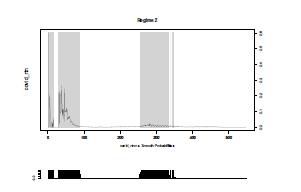
Figure 4: Regime 2 in gray indicates the areas of increasing growth rates

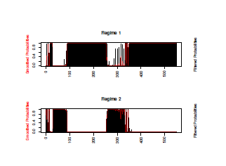
Figure 5: The Smoothed transition probabilities

Figure 4 and 5 display the two switching regimes and their corresponding smoothed transition probabilities, respectively.

The estimated results are summarized in the following Table 4 and 5. Table 4 shows the estimated intercept and its standard error, t value, and Pr(> |t|), and Table 5 gives the estimated transition probabilities, respectively.

Table 4: Estimated intercept and the corresponding statistics

Intercept	Regime 1	Regime 2
Estimate	0.0016	0.0395
Std. Error	0.0001	0.0058
t value	16	6.8103
Pr(> |t|)	2.2e-16 ***	9.7e-12 ***
AIC	-4408.92
Likelihood	2206.46

Table 5: Estimated transition probabilities

Transition probabilities	Regime 1	Regime 2
Regime 1	0.9807	0.0444
Regime 2	0.0193	0.9556

5.3.        Applications of Markov Switching Autoregression Model

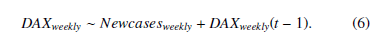
Here we apply the above-mentioned Markov switching autoregressive model of order p to our two data sets. In the following applications, we transform these two daily data sets into weekly ones, namely, DAXweekly, and Newcasesweekly. Application 1: Autoregressive model of order 1 That is to say, we fit the variables as follows.

As a result of this model setting, the following facts are revealed and summarized in Table 6 and 7.

Looking at these tables, it is clear that most of the estimated parameters are statistically significant, except the intercept in Regime 1, and the coefficient of Newcases_weekly in Regime 2.

The multiple R-squared is estimated as 0.8053, and 0.986 in Regime 1 and 2, respectively. Meanwhile, the state transition probabilities are summarized in Table 8. The confidence intervals(CI)(Level= 0.95) for the estimated parameters, namely, intercept, the coefficients of Newcases_weekly and DAX_weekly(t − 1) are displayed in Table 9 and 10.

Table 6: Estimated results of Regime 1

Regime 1	Intercept	Newcasesweekly	DAXweekly(t − 1)
Estimate	1325.08	0.3516	0.8482
Std. Error	1376.41	0.1887	0.1116
t value	0.963	1.8633	7.6004
Pr(> |t|)	0.3357	0.06242 .	2.95e-14***
AIC		1101.393
Likelihood		-544.6966

Table 7: Estimated results of Regime 2

Regime 2	Intercept	Newcasesweekly	DAXweekly(t − 1)
Estimate	521.332	-0.007	0.9700
Std. Error	221.256	0.016	0.0167
t value	2.356	-0.409	58.0838
Pr(> |t|)	0.01846*	0.683	2e-16***

Table 8: Estimated state transition probabilities

	Regime 1	Regime 2
Regime 1	0.6348	0.0852
Regime 2	0.3652	0.9148

Table 9: Confidence intervals for the parameters in Regime 1

	Intercept	Newcasesweekly	DAXweekly(t − 1)
Estimation	1325.0807	0.3516	0.8482
Lower	-1367.0203	-0.0182	0.6298
Upper	4017.1817	0.7214	1.0665

Table 10: Confidence intervals for the parameters in Regime 2

	Intercept	Newcasesweekly	DAXweekly(t − 1)
Estimation	521.3317	-0.0067	0.97
Lower	87.5582	-0.0386	0.937
Upper	955.1051	0.0252	1.0027

These two shifting regimes and their corresponding transition probabilities are displayed in Figure 6 and 7, respectively. Seen from the Figure 6, Regime1(in gray) captures the steep descent of DAX.

As can be seen from the results above, it is clear that, the Markov regime switching autoregressive model of order one captures the sudden ups and downs of the observations. It means that, in the early stages, volatile movements in the market are observed due to the growth of daily new cases, but, after the fortieth day, the change of the stock index slowed down, as if the market had acclimatized to the disease.

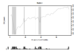
Figure 6: Regime 1(in gray) captures the steep decent of DAX

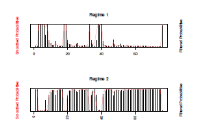
Figure 7: Smoothed transition probabilities

Application 2: Autoregressive model of order 2

We here fit the variables of our data sets by using Markov regime switching autoregressive model of order 2. Namely,

DAXweekly ∼ Newcasesweekly+DAXweekly(t−1)+DAXweekly(t−2).

The numerical results are summarized in Table 11 and Table Seen from these tables, it is clear that most of the estimated statistics are better than the results of AR(1) model obtained above, even the multiple R-Squared is better in each Regime.

	Intercept	Newcasesweekly	DAXweekly(t−1)	DAXweekly(t−2)
Estimate	2642.633	0.367	1.337	-0.584
Std. Error	1365.812	0.170	0.227	0.262
t value	1.935	2.152	5.892	-2.231
Pr(> |t|)	0.0530	0.0314*	3.8e-9***	0.0257*
R-squared		0.857
AIC		1083.065
Likelihood		-533.5325

Table 11: Corresponding statistics of Regime 1

	Intercept	Newcasesweekly	DAXweekly(t−1)	DAXweekly(t−2)
Estimate	586.227	0.0006	0.867	0.098
Std. Error	217.604	0.016	0.078	0.075
t value	2.694	0.038	11.134	1.302
Pr(> |t|)	0.0071**	0.9699	2e-16***	0.193
R-squared		0.9871

Table 12: Corresponding statistics of Regime 2

The estimated state transition probabilities are listed in Table 13.

Table 13: Estimated state transition probabilities

	Regime 1	Regime 2
Regime 1	0.7071	0.0904
Regime 2	0.2929	0.9096

Furthermore, looking at Table 11 , we see that the weekly new cases do have impact on the market, meanwhile DAX_weekly(t-1), DAX_weekly(t-2) show statistically significant in this AR(2) model setting. It also can be confirmed that Figure 8 captures the stock market plunges precisely. In other words, it reveals that Markov Switching Autoregressive Analysis can identify change points precisely as well as other tools, the change point identification based upon a Bayesian approach, for example.

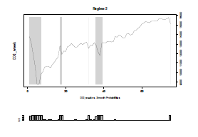
Figure 8: Regime 2(in gray) captures the market plunges

6. Fitting the Datasets Using GARCH Models

In this section, we first fit our two datasets using GARCH models, since GARCH model is considered to be a useful mean for capturing the dynamics in data.The dynamics or the momentum can be described by the volatilities series obtained from GARCH model. Second, we apply MRSA to the volatilities to see whether there exists some sort of co-movement between the weekly growth rates of the disease and the weekly returns of stock index. Details of GARCH model are omitted here, one may get more information from other references, such as, [22], [23]. Hereafter, we just display our empirical results. Our model fittings reveal that GARCH(1,1) and GARCH(1,0) are the best choices for the weekly returns of DAX and the weekly growth rates of the disease.

The plots of weekly stock returns and the weekly number of the newly infected are shown in Figure 9 (leftup) and Figure 10 (leftup) below. It seems that the DAX Index didn’t react sensitively, in corresponding to the changes of the weekly new cases. However, we get completely different results if we fit the weekly stock returns and growth rates using GARCH models, and then apply the Markov regime switching autoregressive model to volatilities obtained from the GARCH model fittings.

6.1.        Fitting Results of DAX Index

By setting different p,q values in GARCH(p,q), we find that GARCH(1,1) fits the weekly DAX returns most appropriately, where returns_weekly = log(r_t) − logr_t−1, where r_t is the price at week t. It indicates the weekly returns follow a skewed normal distribution based upon the numerical results. The fitting results are shown in Table 14. Looking at the table, we see it is a good fit.

Table 14: Summarized results for GARCH(1,1)

	omega	alpha1	beta1	skew
Estimation	4.4675e-05	0.30499	0.70171	0.84704
Std err	3.785e-05	0.1497	0.1032	0.1021
t Value	1.180	2.037	6.798	8.299
Pr(> |t|)	0.2379	0.0416*	1.1e-11***	2e-16***
AIC			-4.0190
BIC			-3.8964
HQIC			-3.9700
Likelihood			-156.72

The original time series of weekly DAX Index, its returns, h_t, and σ_t values obtained from the GARCH(1,1) model, are shown in Figure 9, respectively.

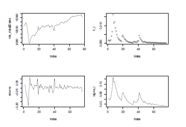
Figure 9: Plots of the results of GARCH(1,1) for returns

It can be confirmed in both Table 14 and Figure 9, that the dynamics of the weekly stock returns is well-captured by GARCH(1,1) model.

6.2.        Fitting Results of Weekly Confirmed Number

Similarly to the DAX index above, we calculate the corresponding weekly growth rates of the disease, namely, growthrate_weekly = logn_t − logn_t−1, where n_t is the number at week t. We then fit the weekly data set using GARCH(p,q) model. By setting different p, q values in the model, we find that GARCH(1,0) fits the weekly growth rates most appropriately.

The fitting results are shown in Table 15. Looking at the table, we see a skewed normal distribution is detected, because of the data’s statistical properties. It indicates that the dynamics of the statistical properties of the data is well captured by a skewed normal distribution. And what is more important is that all the corresponding statistics are statistically significant, a good fit as well.

Table 15: Summarized results for GARCH(1,0)

	omega	alpha1	skewness
Estimate	0.2337	0.2936	1.0158
Std. Error	0.0465	0.1534	0.1322
t value	5.025	1.914	7.685
Pr(> |t|)	5.03e-07***	0.0557.	1.53e-14***

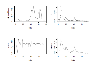
Figure 10: Plots of the results of GARCH(1,0) for growth rates

Similarly, the original time series of weekly number of new cases, weekly growth rates, h_t, and σ_t values obtained from the GARCH(1,0) model, are shown in Figure 10, respectively. It can be confirmed in both Table 15 and Figure 10, that the dynamics of the weekly growth rates is well captured by GARCH(1,0) model.

6.3.        MRSA for Volatilities Obtained from GARCH Models

In order to investigate the linkage and co-movement between the stock returns and the growth rates of the disease, we carry out MRSA based upon (2) using these two volatilities series(σ^return_t ,σ^growthrate_t ), which are obtained from the GARCH(1,1) and the GARCH(1,0) models for the weekly returns and growth rates, respectively.

The estimated results are summarized in Table 16 and 17. And the linkage and co-movement are shown in Figure 11 and 12. Seen from Table 16, the growth rate of the disease, which is regarded as an exogenous variable in the model setting, makes a severe impact on the stock change no matter which regime it stays.

Table 16: Estimated parameters for MRSA

Regime 1	Estimation	Std. Error	t value	Pr(> |t|)
(Intercept)	0.0007	0.0009	0.7778	0.4367
σgrowthratet	0.0031	0.0016	1.9375	0.0527 .
σreturnt−1	0.8264	0.0059	140.068	2e-16***
R-squared		0.9972
Regime 2	Estimation	Std. Error	t value	Pr(> |t|)
(Intercept)	-0.0151	0.0070	-2.1571	0.031*
σgrowthratet	0.0424	0.0107	3.9626	7.4e-05***
σreturnt−1	0.9644	0.1090	8.8477	2.2e-16***
R-squared		0.8972

The estimated state transition probabilities are shown in Table 17.

Table 17: Transition probabilities

	Regime 1	Regime 2
Regime 1	0.8075	0.5387
Regime 2	0.1925	0.4613

The smoothed state transition probabilities are shown in Figure 11, Regime 1(up), and Regime 2(down). And Regime 1 is displayed in Figure 12. It can be seen that the decayed σ_ts of DAX Index are captured in gray(Regime 1). These decayed parts (intervals) are corresponding to the change points as well.

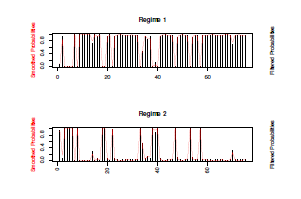
Figure 11: Smoothed state transition probabilities of regimes

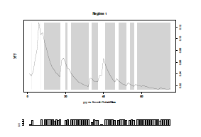
Figure 12: Regime 1 shows the decayed parts of DAX(YYY=σ_t)

Through our numerical analyses, it is confirmed that our proposed the Markov Regime Switching Analysis models are effective in investigating the dynamics, linkage and co-movement between the stock returns and the growth rates of the disease, namely, the statistical characteristics of the data are captured more precisely by using the volatilities obtained from GARCH models.

7. Concluding Remarks

In this paper, we have proposed and employed econometric apparatus and tools, the Markov Regime Switching Analysis method and other methods to investigate the situations of the outbreak of COVID-19 and its impact on German stock market.

It has been confirmed that the dynamics, linkage and comovement between stock returns and growth rates of the disease are well captured by our proposed MRSA models through our numerical analyses.

Moreover, it has been confirmed that it is effective in precisely capturing the linkages between the stock returns and the growth rates of the disease by using volatilities obtained from GRACH models.

Our proposed methods are highly practical, it indicates the possibility of replicating the results obtained in this study to assess the impact of other epidemics and negative factors on economic activities, and provide researchers and policy-makers with a clue of how a pandemic evolved and what impact on the economies. It may lead to better measures and actions while dealing with another pandemic in the future.

Acknowledgment

The authors are grateful to the reviewers’ valuable comments that improved the manuscript. This study was partly supported by the Japan Society for the Promotion of Science(JSPS) KAKENHI Grant Number(c)18K04626. The authors would like to thank the organization.

1. K.R. Tan, S. Tokinaga, “Markov Regime Switching Analysis for the Pandemic and the Dynamics of German Market,” Proceedings of International Conference on Computational Science and Computational Intelligence(CSCI), IEEE Xplore, 2021.
2. D.W.K. Andrews, “Tests for parameter instability and structural change with unknown change points,” Econometrica, 61, 821-856, 1993.
3. J. Chen, A.K. Gupta, “Change point analysis of a Gaussian model,” Statistical Papers, 40, 323-333, 1999.
4. F. Desobry, M. Davy, C. Doncarli, “An online kernel change detection algorithm,” IEEE Trans. Signal Process, 53(8), 2961-2974, 2005.
5. G. Koop, S.M. Potter, “Estimation and forecasting in models with multiple breaks,” Review of Economic Studies, 74(3), 763-789, 2007.
6. R. Malladi, G.P. Kalamangalam, B. Aazhang, “Online Bayesian Change Point Detection Algorithms for Segmentation of Epileptic Activity,” Asilomar Conference on Signals, Systems and Computers, 1833-1837, 2013.
7. J. Knoblauch, T. Damoulas, “Spatio-temporal Bayesian On-line Changepoint Detection with Model Selection,” Proceedings of the 35th International Conference on Machine Learning(ICML-18), 2718-2727, 2018.
8. K.R. Tan, “Detecting structural changes in stochastic differential equation system based upon a Bayesian approach,” Journal of Economic and Social Research, 58(1-2), 51-67, 2018.
9. K.R. Tan, “Identifying the pandemic change points of COVID-19 outbreak: case studies in Germany, Italy and Austria,” Journal of Economic and Social
   Research, 61(2-3), 19-33, 2021.
10. S. Tokinaga, S. Matsuno, “Estimation of Transition of Credit Rating by Using Particle Filters Based on State Equations Approximated by the Genetic Programming,” IEICE Proceeding Series, 45, 397-400, 2011.
11. F. Caron, A. Doucet, R. Gottardo, “On-line changepoint detection and parameter estimation with application to genomic data,” Stat Comput, 22, 579-595, 2012.
12. J.D. Hamilton, “Rational-expectations econometric analysis of changes in regimes: an investigation of the term structure of interest rates,” Journal of Economic Dynamics and Control, 12, 385-423, 1998.
13. J.D. Hamilton, “A new approach to the economic analysis of nonstationary time series and the business cycle,” Econometrica, 57, 357-384, 1989.
14. J.D. Hamilton, Time series analysis, Princeton University Press, 1994.
15. S. Goutte, B. Zou, “Foreign exchange rates under Markov regime switching model,” Center for Research in Economic Analysis Discussion Paper, 16, 1-29, 2011.
16. A. Ramponi, “VaR-optimal risk management in regime-switching jump- diffusion models,” Journal of Mathematical Finance, 3(1), 103-109, 2013.
17. S. Choi, M. Marcozzi, “A regime switching model for the term structure of credit risk spreads,” Journal of Mathematical Finance, 5, 49-57, 2015.
18. H. Boubaker, N. Sghaier, “Markov-switching time-varying copula modeling of dependence structure between oil and GCC stock markets,” Open Journal of Statistics, 6, 565-589, 2016.
19. S. Gyamerah, P. Ngare, “Regime-switching model on hourly electricity spot price dynamics,” Journal of Mathematical Finance, 8, 102-110, 2018.
20. G. Stefano, O. Aydin, S. Abhijit, J. Mazin, “Pricing of time-varying illiquidity within the Eurozone: evidence using a Markov switching liquidity-adjusted capital asset pricing model,” International Review of Financial Analysis, 64, 145-158, 2019.
21. Z. Qu, Z. Fan, “Likelihood ratio-based tests for Markov regime switching,” Review of Economic Studies, 88(2), 937-968, 2021.
22. R. Engle, “Autoregressive conditional heteroscedasticity with estimates of the variance of United Kingdom inflation,” Econometrica, 50, 987-1007, 1982.
23. T. Bollerslev, “Generalized autoregressive conditional heteroskedasticity,” Econometrics, 31, 307-327, 1986.
24. P. Yu, T. Liu, Q. Ding, “Volatility analysis of web news and public attitude by GARCH model,” Psychology, 3, 610-612, 2012.
25. C. Dritsaki, “An empirical evaluation in GARCH volatility modeling: evidence from the Stockholm stock exchange,” Journal of Mathematical Finance, 7, 366-390, 2017.
26. W. Zhang, P. Yang, “Research on dynamic relationship between exchange rate and stock price based on GARCH-in-mean model,” Journal of Service Science and Management, 11, 691-702, 2018.
27. A. Ngunyi, S. Mundia, C. Omari, “Modelling volatility dynamics of cryptocurrencies using GARCH models,” Journal of Mathematical Finance, 9, 591-615,2019.

(Click Here)