1. Introduction

In a world that is becoming increasingly and wirelessly connected, network security is now a critical task that must be seriously considered. It is necessary to avoid cybercriminals gaining illegal access to valuable data and sensitive information. It is important to note that the amount of data that devices produce, and the number of resources used, increase as more devices are connected. When an unauthorized user gets hold of data, he can cause several problems such as stolen assets, identity theft and reputational damage – not only to the individual but also to the entire network. A vulnerability can be described as a situation where a subject A (item, process or person) manages to exploit the privileges of a subject B to carry out operations not initially granted to him. Therefore, it is necessary to proactively manage risks, threats, and vulnerabilities.

Many studies have recently focused on Information Technology (IT) resilience. It describes the ability of a system to continue to deliver the expected results despite the occurrence of incidents, such as natural disasters and especially cyber-attacks.

In this scenario, Internet of Things (IoT) devices are particularly vulnerable to network attacks and the situation becomes extremely dangerous when we consider e-health devices. E-health data represents one of the most important personal information. It is important to design the system as confidential as possible, with high-level security policies. Even if various regulations for data management have been drafted over the years – such as the General Data Protection Regulation (GDPR, https://gdpr-info.eu/) – it is not uncommon to read news of improper exfiltration of data by unauthorized users: according to Protenus Breach Barometer, in 2022 there were 50M+ Patient records breached, 905 Incidents, 44% Increase in hacking incidents (https://www.protenus.com/breach-barometer-report).

The Internet of Medical Things (IoMT) [1] is that set of technologies aimed at using smart devices – connected to each other, even via the internet – in the medical field. If this technology guarantees an improvement in healthcare management, on the other hand new security challenges are expected: it is necessary to ensure correct authentication and authorization procedures (applying minimum privilege as much as possible), maintaining the confidentiality of data (both at rest and in transit, with encryption and obfuscation techniques) and integrity (making sure that the data is not modified by malicious users).

For obtain confidential communications, cryptography is used. It is a technique for encoding messages: symmetric encryption is based on sharing a shared secret; asymmetric cryptography is based on a pair of keys – public key and private key – used respectively to sign a message and to verify its integrity [2] . Given the low computing power, the encryption algorithms used in the IoMT are different from those used in servers, and they are classified into three categories: centralized (i), non-centralized (ii), low weight (iii) [3]. The centralized approach (i) uses a central node – often a server and not an IoT device – to encrypt the message. The sender sends the message in clear text over a secure channel to the centralized server which encrypts it and sends it over the potentially insecure channel to the receiver. The central node requires a lot of computing power, and it is a single point of failure (see Figure 1).

In the decentralized approach (ii) the encryption is distributed on the various link-by-link nodes: one node receives the encrypted message, decrypts it, re-encrypts it and transmits it to the next node. There is additional encryption level between end systems (see Figure 2).

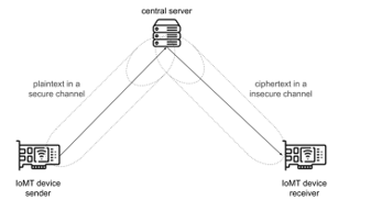
Figure 1: Centralized approach in IoMT cryptography

To minimize the effort of the devices, over the years various approaches have been proposed which are based on symmetric encryption in which each network node authenticates the others [4]. These algorithms belong to the low weight security approach (iii).

Obfuscation techniques, in accordance with the principles of least privilege, aim to make data inaccessible when it is not needed. Unlike encryption algorithms that use a key, to understand the plaintext you only need to know the algorithm for generating the obfuscated data [5]. More sophisticated techniques allow to completely anonymize the data, no longer allowing the re-identification of the data after anonymization [6].

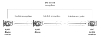
Figure 2: Decentralized approach in IoMT cryptography

The techniques and attacks used by hackers to compromise a system have become increasingly sophisticated so that human observation is less and less useful in identifying a compromise.

It is precisely here that Machine Learning (ML) in cybersecurity comes into play: in fact, the use of ML lends itself greatly to solving this type of problem. The systems can analyze patterns and learn from them to help prevent similar attacks and respond to behavior change. Generalization is the capacity of an ML model to fit correctly to additional, previously unobserved data taken from the same distribution as the model’s original data. Because ML can learn from past data, it can recognize odd communications and user behaviors. As a result, it is possible to prevent threats and respond to active attacks in real time, not only reducing the amount of time spent on routine tasks but also allowing us to use the network’s resources more strategically.

Artificial Intelligence (AI) approaches are widely used in healthcare: to preserve the privacy of health data from access by unauthorized users, several frameworks have been proposed for analyzing user behavior in a secure environment. Behavioral anomalies – such as unusual login and actions – are flagged by the system as suspicious and blocked [7]. Several vendors – e.g., Microsoft and Google – have implemented these security systems called Security Information and Event Management (SIEM). They are capable of monitoring and identify possible vulnerabilities and acting to mitigate them. Each SIEM is always composed of at least three main modules which are data collection (i), learning the normal flow without malicious actions (ii) and generating the classification report (iii) [8].

Over the years SIEM’s training baseline has evolved, moving from using legacy Machine Learning models (e.g., Support Vector Machine, Decision Tree, K-NN [9]) to using Deep Learning (DL) models [10]: researchers have proposed systems running MLP-based Neural Networks [11], DNNs with optimization techniques (Principal Component Analysis and Gray Wolf Optimization) [12], Convolutional Neural Networks with Long Short-Term Memory [13].

Cyberattacks from malicious users are increasingly accurate and range across the entire ISO-OSI stack: Perception-level attacks can involve Denial of Service (DoD) of physical devices or RFID spoofing and cloning; Application layer attacks can create a Man in The Middle (active or passive) by sniffing network traffic by installing Malware or Medical information injections. At network level, attackers can invalidate DNS or ARP tables to redirect traffic to their destinations [14]. In this scenario, Covert Channels (CC) assume a great importance. Covert Channels are channels used to transmit information using existing system resources that were not designed to carry data. They make it possible not to show the communication taking place between two interlocutors in order not to alarm a third agent – potentially malicious and looking to exfiltrate data. The main characteristics of a CC are stealthies, low bandwidth and indistinguishability. Due to their ability to evade detection, they pose a serious threat to cyber security because attackers can use them for malicious scopes [15]. There are various types of Covert Channels: Covert Timing Channel (i), Covert Storage Channel (ii), Covert Behavioral Channel (iii). Covert Timing Channels (i) use a time measurement to signal the value to be sent on the channel; Covert Storage Channels (ii) encode information by hiding it in the fields of the network protocol used; Covert Behavioral Channels (iii) divide the hidden message to be sent and transmit it in smaller packets and generally using a lower-level protocol.

More recently, ML and statistical methods for detecting CTC attacks communications were presented such as temporal analysis (i), traffic analysis on the channel (ii), the observation of side channels (iii) and the study of entropy (iv).

In the temporal analysis (i), the computing times of the devices are analyzed to identify any anomalies: if the response time of a device varies abruptly, the presence of a CTC involving that device can be assumed. Unfortunately, this approach is subject to jitter: legitimate traffic on the channel stresses the devices and a false CTC alarm can be raised [16].

The traffic analysis on channel (ii) analyzes the traffic but takes into account factors like the frequency of packet sending, their volume, and occasionally even their content. By gathering the network traffic exchanged, a statistical model of the system is constructed in a secure environment, and from these the significant communication frequencies are discovered. The network traffic is evaluated in the detection phase, and the presence of a CTC can be suspected if there are several significant frequencies [17].

The execution of Covert Channels has unintended consequences for the systems; the variation of the side channels can be investigated (iii) to spot any network anomalies like CTC attacks. It is extremely challenging to isolate the various processes from one another in a system with highly interconnected components. A message exchange over unconventional channels is referred to as a CC when both the sender and the recipient are aware of it, and a SC when the message is sent by the sender involuntarily, such as through cache access, data movement between the CPU and memory, or the processor emitting electromagnetic waves. The identification of CCs by SC is still under study and there is no proof of its correctness [18].

The system’s entropy can be affected by a CTC, and as a result, this measurement can offer helpful information for detection. Information Theory uses entropy as a metric to quantify the degree of disorder or uncertainty in a system. Entropy is a measure of how random and erratic messages are exchanged in the network about the problem of detecting a Covert Timing Channel. A legitimate communication system, as opposed to one that sends messages according to a set of rules and behaviors (such as the CTC-TR), is unpredictable and has a high degree of entropy. In [19], the authors demonstrate a method based on entropy (iv) using conditional entropy, which is an estimation of the system’s entropy’s value obtained from available data.

In recent years, ML models have been used in Covert Timing Channel identification systems: starting with network traffic that has been detected and then being cleaned up by removing unnecessary data, AI models are trained on the resulting data. KNN, SVM, and Naive Bayes are three of the most popular ML models [20].

With the aid of VGG-16 and Squeeze Net, the first instances of the application of DL approaches for the identification of CTCs and their validity can be seen [21].

In this paper, the hidden communication is embedded in the legitimate traffic by means of a CTC, obtained by modulating the inter-arrival packet delays. In practice, the malicious process modulates the inter-arrival delay of the transmitted e-health data, by transmitting one 0 bit (or 1 bit) when the delay is less (greater) than a pre-defined threshold. Here, we move one step further by proposing a type of CTC, based on the inter-arrival delays of TCP packets. In addition, we implement an ML and DL framework to detect what kind of message is transmitted on the channel in CTC (see Figure 3).

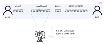
Figure 3: CTC scenario under consideration

The obtained results thus confirm the validity of such approach for ML and DL detection of hidden communications – the current State of Art in detecting CTCs is based on the analysis of the statistical variation of traffic on the network: as soon as this changes and exceeds a chosen threshold, an alert of a possible attack is sent; unfortunately this approach fails to detect highly stealthy traffic: a CTC uses the same throughput as the legitimate communication channel. For this reason, a DL model that can capture the insight hidden in the channel itself is needed.

The remainder of our work is organized as follows. Section 2 illustrates a Covert Timing Channel model and how the dataset of hidden communications is generated. Section 3 shows the ML and DL methods used for the detection of illegitimate traffic, while Section 4 discusses the simulation results and shows the performance of the methods according to the main metrics used for evaluating the proposed pipeline.

2. Covert Timing Channel and Dataset Generation

 For simplicity, we indicate two interlocutors as Alice and Bob. They establish a CTC communication. There is also a third user on the channel, Cindy, who is listening and has the aim of recovering the type of message that Alice and Bob are exchanging (see Figure 4). Let’s consider Alice as a user with an active role in the communication: she is the only one who sends messages in the channel, while Bob is listening for them. It’s not hard to think a real-life use case where an edge device sends messages to a central system hub to notify an event.

To understand how this channel works, it is necessary to start from a basic concept: what Alice sends on the channel is completely unrelated to what she is communicating. What’s really related is how Alice is sending the message. As previously described, in a CTC the message is encoded in the packet interarrival time. We therefore distinguish between a covering message and a covered message: the first one is the message that Cindy recovers by sniffing the traffic, the second is the one that only Bob can reconstruct.

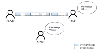
Figure 4: Scenario under consideration

Let’s see how it is possible to encode the message that Alice wants to send using the packet interarrival times. Let  be the message to send. The first operation that Alice performs is the conversion of  into binary: each ASCII character can be represented using -bit sequence according to Table 1.

Table 1: Encoding ASCII to 7 bits string

	Leftmost three bits
Righmost four bits	000	001	010	011	100	101	110	111
0000	NUL	DLE	Space	0	@	P	’	p
0001	SOH	DC1	!	1	A	Q	a	q
0010	STX	DC2	“	2	B	R	b	r
0011	ETX	DC3	#	3	C	S	c	s
0100	EOT	DC4	$	4	D	T	d	t
0101	ENQ	NAK	%	5	E	U	e	u
0110	ACK	SYN	&	6	F	V	f	v
0111	BEL	ETB	‘	7	G	W	g	w
1000	BS	CAN	(	8	H	X	h	x
1001	HT	EM	)	9	I	Y	i	y
1010	VF	SUB	*	:	J	Z	j	z
1011	VT	ESC	+	;	K	[	k	{
1100	FF	FS	,	<	L	\	l	|
1101	CR	GS	–	=	M	]	m	}
1110	SO	RS	.	>	N	^	n	~
1111	SI	US	/	?	O	_	o	DEL

Let  be the binary string representing . Note that  will be  times the length of the initial string . At this time  packets will be sent on the channel – one for each bit of . Each packet will be sent waiting a specifying time after the previous depending on whether we want to send a  bit or a  bit (e.g.,  waiting  milliseconds,  waiting  milliseconds). It is necessary to have a specific packet to notify the beginning and the ending of the message.

The packets sent by Alice are simple TCP frame for communication at level  of the ISO-OSI stack and each of them contains a character of the covering message. It is obvious that the more the covering message makes sense, the less Cindy will be suspicious of the presence of a hidden communication between Alice and Bob.

Note that if the  is shorter than the message to be sent, it must be repeated several times to cover completely it (see Figure 5).

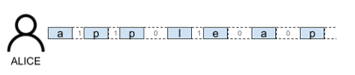
Figure 5: Example of CTC messaging packets

The use case we have considered is the one where an edge device notifies to a central hub several messages relating to events of 4 different kinds: the request to generate an access token for a user starting from the  or , checking the validity of a  or a  used as heartbeat. For simplicity, both the edge device and the central hub are active on the same LAN by establishing a socket between them.

We created a dataset with  types of messages (see Table 2), developing the CTC described using python and sniffing communication using Wireshark.

Our analysis did not focus on internal packet analysis (known as ) but rather we considered packet interarrival time as a classification vector. Considering the interarrival times of the packets we have created the representative spectrograms of the communications [22]. To produce the spectrograms, the packet interarrival times were collected and considered as sampling instants of a chirp signal. A chirp signal has the characteristic that its frequency varies – increasing or decreasing – over time. A linear increase was considered. The Short-Time Fourier Transform ( ) was applied to the chirp signal, obtaining a matrix representation in which each column contains an estimate of the short-term frequency content located in the time of the signal itself. The matrix is the spectrogram of the communication encoded in RGB space. Each communication is therefore not represented by a flow of packets but by a single spectrogram which contains its characteristics (Figure 6).

Table 2. Number of instances for each class

The input for Deep Learning models described later will be images of the size  and for our experiment we divided it in training set and test set with  ratio.

Figure 6: Example of Spectrogram

3. Machine and Deep Learning Models

Over the years several Machine Learning models have been proposed for the classification task and some of them have been considered for our experiments.

We have implemented the following models.

• (Figure 7)
• – (see Figure 8)
• (Figure 9)
• (Figure10)

The  model is based on the construction of several  – other classification models – and the final output is obtained by combining the outputs of the individual s by applying the majority vote approach. A  is a tree whose internal nodes represent feature splits, and the leaves represent classes. The idea is to traverse the tree from the root and based by values of the instance to classify and the node splits arrive on a leaf node and assign the corresponding class. To decide how to create the tree – such as which feature use at which level – are used different criteria such as entropy, information gain and Gini index.

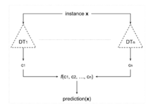
Figure 7: Schema of Random Forest model

To better understand how –  works it is necessary to introduce the . The idea of the  is very simple:  instances of the same class are very similar to each other. Similarity can be calculated as the distance – consider the  distance – between the vectorial representations of the two instances. To classify an input, therefore, it is sufficient to retrieve the item closest to it and assign it the same class.  retrieves the  closest items and assigns to the input the class that has majority votes.

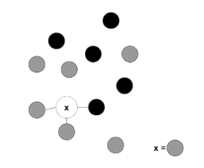
Figure 8: Example of K-NN prediction

A Convolutional Neural Network is a particular type of artificial neural network ( ) widely used for many visual tasks such as image recognition, object classification and pattern recognition. It is composed in sequence of – at least – three types of layers: Convolution Layer (or Kernel), Pooling Layer and Fully Connected Layer. In the Convolutional Layer the image (a matrix of pixels) is input and a smaller matrix than the starting one is output. The output matrix is obtained by sliding an activation map over the input matrix and applying the dot product between it and the selected portion of the image. The goal of the pooling layer is to reduce the spatial dimension of the representation by extracting the dominant features. In the Fully connected layer, we try to learn non-linear combinations of the characteristics of the representation obtained. The Fully Connected level is trying to learn the nonlinear function that connects input to output.

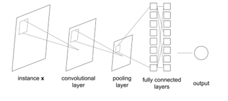
Figure 9: General schema of a CNN

A Convolutional Siamese Network [23] has two images as input and returns the similarity between them. Internally it is composed of two – or more –  that share the same weights. When classifying an image with a convolutional network the last layer is almost always a layer with a SoftMax function: we obtain a vector of  elements, and  contains the probability of confidentiality in assigning class i to the image of inputs.

In a Siamese Network the last layer is eliminated, and another one is added to calculate the difference between the two representations. The last level is a single neuron with a sigmoid activation function (  to ).

Figure 10: Siamese Network using CNNs

4. Results

To evaluate the performance of the system, some of the metrics mainly considered were used: , , – ,  and , that are calculated using True ( ) or False ( ) Positive ( ) or Negative ( ). A correctly classified instance is a True Positive; a misclassified instance can be a False Negative or a False Positive. Considering the  class as Positive class: a spectrogram of a credit card is a True Positive if the system assigns it the  class; a spectrogram of a name and surname is a False Positive if the system assigns it the  class; a credit card spectrogram is a False Negative if the system does not assign it the  class.

These values can be obtained by considering the confusion matrix in Table 3.

Table 3: Confusion Matrix of a binary classification

 – as the name suggests – describes how accurate the system is in identifying true positives. If the system has high precision, it means that it is rarely wrong in identifying class of spectrogram: when the system claims the spectrogram is about email information, that is it.

 indicates the ratio of positive instances that are identified by the system. If the system has high recall about  messages, it means that almost all instances about this type of communication have been identified.

–  combines precision and recall into a single metric. This metric is the harmonic mean between the two.

 indicates how close a predicted value is to the actual one: informally, it is the fraction of predictions that are accurate.

 measures the proportion of true negatives and indicates the proportion of truly negative instances that are correctly identified. High specificity means that the model is correctly identifying most negative instances.

Using the , it was possible to identify the optimal value of  in the  algorithm. A similar method was applied to understand the maximum depth value ( ) of the decision trees constructed for the  model.

The best performances were achieved considering the application of an ensemble learning technique called Stacking (STC): the idea is to build a meta-classifier that learns from the classifications of the individual classifiers using a personal weight matrix. The meta classifier uses [24].

The Convolutional Neural Network was built with a single convolutional layer inside it. The input of size  first crosses the convolutional layer characterized by 16 feature maps of size . The new matrix is then computed by the  layer characterized by matrices of size . To minimize overfitting a Dropout layer is then applied with a percentage of  – at each passage of the training data some random nodes are chosen, and they don’t update their weights both in forward and backpropagation. The last layers are composed by a full  layer of  units which is converted to one of length  by the . Using this configuration, the following performances were achieved (see Figure 11).

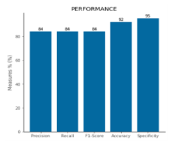
Figure 11: Performance of described CNN

The confusion matrix shows how generally the accuracy is high for all classes and there is no evidence of the imbalance between them. It is important to note the misclassification among  and  classes (see Figure 12).

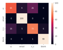
Figure 12: Confusion Matrix of described CNN

Even if the performance of the Neural Network is slightly lower than the application of ensemble techniques, it is very robust to noise. Due to the construction of the Covert Timing Channel and the dataset, the communications are noise-free: we have applied Gaussian noise to the images (see Figure 13).

Figure 13: Noise effect with several Standard Deviation

Gaussian noise is statistical noise having a probability density function equal to that of the normal distribution. We analysed how the performance varies as the standard deviation value of the noise varies (see Figure 14).

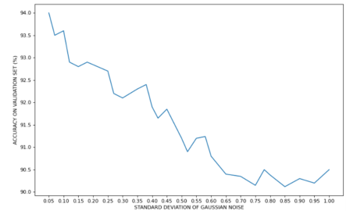
Figure 14: CNN Accuracy, based on Standard Deviation of Gaussian Noise

By testing the results of the various approaches introduced previously – RF, KNN, STC – the convolutional network is the one that maintains the highest accuracy value even in the case of spectrograms strongly affected by noise. It was therefore decided to use CNN as the first model in the classification pipeline (see Figure 15).

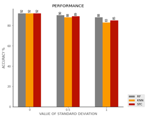
Figure15: Accuracy of ML and DL with several Standard Deviation

To try to improve the performance of Convolutional Neural Network we analysed a Siamese Neural Network. As we can check observing confusion matrix, the network didn’t learn the difference between  and  instances. We trained the network using an input that is constituted by a pair of images. This network consists of two identical subnets that share weights during training. The idea is to train it to understand the level of similarity between two inputs. Internal networks feature a first layer of  which modifies the input tensor. Then, there are  convolutional layers characterized by a dimension of the convolutional kernel equal to  and pairs  respectively ,  and . Relu is used as activation function followed by two layers of .

To easily understand how this network works it is sufficient to think in the following way: two images cross the two internal networks simultaneously and these produce a vectorial representation of them. We calculate the vector distance between them and with a sigmoid neuron we return  or  –  if the images are similar,  otherwise. There are several loss functions for training and in our case  was used.

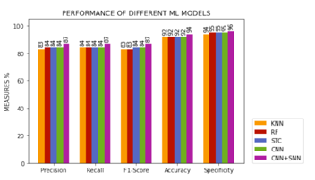
Figure 16: Performance of described ML and DL Models

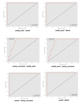
Figure 17: Binary ROCs of proposed pipeline

Once we obtained a very performing Siamese network to discriminate between two classes, it is used it in the following way [24]: we recovered the most significant spectrograms of each class by applying Means, and we built the dissimilarity space with which we trained a  model. The idea is to apply the Neural Network and this new model in cascade: when the  predicts in output that the instance is a  or , then the  and the Siamese Neural Network are asked for confirmation. Using this trick, accuracy improved by two percentage points (see Figure 16).

The value of the AUC – Area Under the Curve – was examined in addition to the metrics previously mentioned. The area under the ROC curve (AUC) is a measurement of its size. The trend of True Positives as a function of False Positives is displayed on a ROC curve – Receiver Operating Characteristics – with different threshold values. In the case of a binary classification, a sigmoid CNN generates a real value in the range : based on a selected threshold, the network determines how to classify the input instance.

AUC measures the classifier’s ability to distinguish between Positive and Negative classes: the higher the AUC, the more effective the model. It is useful to understand how True Positives and False Positives change depending on the chosen threshold.  (True Positive Rate) and  (False Positive Rate) are the two metrics that are used:  is the decrease in Specificity compared to 1 while the  is the same as the Recall.
Figure 17 shows ROC curves in binary classifications.

5. Conclusion

This paper showed how to create a simple CTC and how it is possible to apply Machine Learning (Random Forest and K-NN) and Deep Learning (Convolutional Neural Network and Siamese Network) approaches to classify hidden communications in TCP-based Covert Timing Channels in the e-health field. We proposed an innovative pipeline composed of a single CNN and a SNN to improve the accuracy of the classification. We have compared the performances of different methods and improved them with ensemble and combination techniques. The best performance was achieved by our pipeline with an accuracy of . Even if the performances presented are slightly lower than those of the State of Art – which use ML and statistical models obtaining performances of  [20] – the work paves the way for the use of DL models for the identification of CTCs. The further contribution presented is the noise resistance of the pipeline: if there is noise, modelled with Gaussian distribution and different value of standard deviation applied to spectrograms, the pipeline performance remains efficient with  accuracy.
The detection of the prototypes of each class demonstrates how it is possible to identify a representative spectrogram of each message in transit in the CTC. The prototype can be thought as a hashing of the attack and can be used in SIEM systems to compare the state of the network against each known hashed attack type.The current model has been tested on simple messages: as the number of classes increases, the size of the dissimilarity space increases, which could lead to longer training and identification times. At the same time, the simulated noise is only fictitious: it was inserted afterwards.

We are satisfied with the performances obtained in general but not so much with those relating to the Siamese network. Our future studies will focus on the study of this network and how to combine it with other DL models. Other studies are focusing on the internal analysis of the packets exchanged and using different CTCs.

1. F. Hu, D. Xie, S. Shen, “On the Application of the Internet of Things in the Field of Medical and Health Care,” in 2013 IEEE International Conference on Green Computing and Communications and IEEE Internet of Things and IEEE Cyber, Physical and Social Computing, IEEE: 2053–2058, 2013, doi:10.1109/GreenCom-iThings-CPSCom.2013.384.
2. G.J. Simmons, “Symmetric and Asymmetric Encryption,” ACM Computing Surveys, 11(4), 305–330, 1979, doi:10.1145/356789.356793.
3. S.K. Kharroub, K. Abualsaud, M. Guizani, “Medical IoT: A Comprehensive Survey of Different Encryption and Security Techniques,” in 2020 International Wireless Communications and Mobile Computing (IWCMC), IEEE: 1891–1896, 2020, doi:10.1109/IWCMC48107.2020.9148287.
4. Y. Sun, F.P.-W. Lo, B. Lo, “Lightweight Internet of Things Device Authentication, Encryption, and Key Distribution Using End-to-End Neural Cryptosystems,” IEEE Internet of Things Journal, 9(16), 14978–14987, 2022, doi:10.1109/JIOT.2021.3067036.
5. S.S. Albouq, A.A.A. Sen, A. Namoun, N.M. Bahbouh, A.B. Alkhodre, A. Alshanqiti, “A Double Obfuscation Approach for Protecting the Privacy of IoT Location Based Applications,” IEEE Access, 8, 129415–129431, 2020, doi:10.1109/ACCESS.2020.3009200.
6. L. SWEENEY, “k-ANONYMITY: A MODEL FOR PROTECTING PRIVACY,” International Journal of Uncertainty, Fuzziness and Knowledge-Based Systems, 10(05), 557–570, 2002, doi:10.1142/S0218488502001648.
7. A. Sundas, S. Badotra, S. Bharany, A. Almogren, E.M. Tag-ElDin, A.U. Rehman, “HealthGuard: An Intelligent Healthcare System Security Framework Based on Machine Learning,” Sustainability, 14(19), 11934, 2022, doi:10.3390/su141911934.
8. J. Asharf, N. Moustafa, H. Khurshid, E. Debie, W. Haider, A. Wahab, “A Review of Intrusion Detection Systems Using Machine and Deep Learning in Internet of Things: Challenges, Solutions and Future Directions,” Electronics, 9(7), 1177, 2020, doi:10.3390/electronics9071177.
9. C. Janiesch, P. Zschech, K. Heinrich, “Machine learning and deep learning,” Electronic Markets, 31(3), 685–695, 2021, doi:10.1007/s12525-021-00475-2.
10. Y. Rbah, M. Mahfoudi, Y. Balboul, M. Fattah, S. Mazer, M. Elbekkali, B. Bernoussi, “Machine Learning and Deep Learning Methods for Intrusion Detection Systems in IoMT: A survey,” in 2022 2nd International Conference on Innovative Research in Applied Science, Engineering and Technology (IRASET), IEEE: 1–9, 2022, doi:10.1109/IRASET52964.2022.9738218.
11. H. Rathore, L. Wenzel, A.K. Al-Ali, A. Mohamed, X. Du, M. Guizani, “Multi-Layer Perceptron Model on Chip for Secure Diabetic Treatment,” IEEE Access, 6, 44718–44730, 2018, doi:10.1109/ACCESS.2018.2854822.
12. S.P. R.M., P.K.R. Maddikunta, P. M., S. Koppu, T.R. Gadekallu, C.L. Chowdhary, M. Alazab, “An effective feature engineering for DNN using hybrid PCA-GWO for intrusion detection in IoMT architecture,” Computer Communications, 160, 139–149, 2020, doi:10.1016/j.comcom.2020.05.048.
13. S. Khan, A. Akhunzada, “A hybrid DL-driven intelligent SDN-enabled malware detection framework for Internet of Medical Things (IoMT),” Computer Communications, 170, 209–216, 2021, doi:10.1016/j.comcom.2021.01.013.
14. A. Djenna, D. Eddine Saidouni, “Cyber Attacks Classification in IoT-Based-Healthcare Infrastructure,” in 2018 2nd Cyber Security in Networking Conference (CSNet), IEEE: 1–4, 2018, doi:10.1109/CSNET.2018.8602974.
15. H. Okhravi, S. Bak, S.T. King, “Design, implementation and evaluation of covert channel attacks,” in 2010 IEEE International Conference on Technologies for Homeland Security (HST), IEEE: 481–487, 2010, doi:10.1109/THS.2010.5654967.
16. A. Chen, W.B. Moore, H. Xiao, A. Haeberlen, L. Thi Xuan Phan, M. Sherr, W.Z. Zhou, Detecting Covert Timing Channels with Time-Deterministic Replay, USENIX Association, 2014.
17. F. Chen, Y. Wang, H. Song, X. Li, “A statistical study of covert timing channels using network packet frequency,” in 2015 IEEE International Conference on Intelligence and Security Informatics (ISI), IEEE: 166–168, 2015, doi:10.1109/ISI.2015.7165963.
18. C. Shepherd, J. Kalbantner, B. Semal, K. Markantonakis, “A Side-channel Analysis of Sensor Multiplexing for Covert Channels and Application Fingerprinting on Mobile Devices,” 2021.
19. S. Gianvecchio, Haining Wang, “An Entropy-Based Approach to Detecting Covert Timing Channels,” IEEE Transactions on Dependable and Secure Computing, 8(6), 785–797, 2011, doi:10.1109/TDSC.2010.46.
20. M.A. Elsadig, A. Gafar, “Covert Channel Detection: Machine Learning Approaches,” IEEE Access, 10, 38391–38405, 2022, doi:10.1109/ACCESS.2022.3164392.
21. F. Massimi, F. Benedetto, “Deep Learning-based Detection Methods for Covert Communications in E- Health Transmissions,” in 2022 45th International Conference on Telecommunications and Signal Processing (TSP), IEEE: 11–16, 2022, doi:10.1109/TSP55681.2022.9851366.
22. S. Al-Eidi, O. Darwish, Y. Chen, G. Husari, “SnapCatch: Automatic Detection of Covert Timing Channels Using Image Processing and Machine Learning,” IEEE Access, 9, 177–191, 2021, doi:10.1109/ACCESS.2020.3046234.
23. J. BROMLEY, J.W. BENTZ, L. BOTTOU, I. GUYON, Y. LECUN, C. MOORE, E. SÄCKINGER, R. SHAH, “SIGNATURE VERIFICATION USING A ‘SIAMESE’ TIME DELAY NEURAL NETWORK,” International Journal of Pattern Recognition and Artificial Intelligence, 07(04), 669–688, 1993, doi:10.1142/S0218001493000339.
24. T.N. Rincy, R. Gupta, “Ensemble Learning Techniques and its Efficiency in Machine Learning: A Survey,” in 2nd International Conference on Data, Engineering and Applications (IDEA), IEEE: 1–6, 2020, doi:10.1109/IDEA49133.2020.9170675.

(Click Here)