1. Introduction

The field of human resources (HR) has undergone significant changes over the past few decades, and the rise of artificial intelligence (AI) has had a major impact on how HR functions are performed. From recruitment and employee evaluation to training and career development, the introduction of AI has led to a transformation in the way HR professionals perform their duties. This article will delve into the literature on the impact of AI in HR, analyzing the advantages and drawbacks of utilizing AI in this field, and examining the potential implications for HR professionals and organizations.

Another area where AI is having an impact is in employee evaluation and performance management. AI algorithms can analyze an employee’s work history, skills, and achievements to predict their potential for growth and future success within the company. This can help HR professionals make informed decisions about employee development and career advancement. For example, in a study by Deloitte, 92% of HR professionals reported that AI has improved the accuracy of performance evaluations (Deloitte, 2019). Performance job prediction has become increasingly popular with the advent of machine learning algorithms such as decision trees, random forests, and support vector machines, which can handle vast quantities of data and discern intricate connections between various variables. These algorithms can be trained on historical performance data to make predictions about the future performance of new hires or current employees. In this study, we will focus on the application of the ANN on the candidates performance prediction [1].

Designing an ANN with the appropriate parameters can result in a powerful tool. In fact, the process of choosing selecting the architecture that will works well includes the number of input, hidden neurons and weight values, for a complex situations can pose an optimization task challenge. The training process plays a crucial role in determining the ANN topology. Firstly, the most suitable architecture needs to be chosen by assessing the problem at hand, which entails identifying the number of input, hidden, and output neurons. Secondly, the ideal weight values that enable the ANN model to perform at its best must be identified. While the ANN architecture is typically determined by experience, some researchers have started using meta-heuristic algorithms such as Particle Swarm Optimization to explore various possible architectures and select the optimal one based on a fitness criterion.

The primary objective of this study is to create a job performance prediction model that utilizes ANN, PSO, and appropriately selected variables based on the availability of data. The first step involves examining the effectiveness of variable selection models by comparing discriminant analysis and logistic regression techniques. The second step entails identifying the optimal ANN topology by proposing a training process that employs the PSO algorithm to determine the ideal neural network topology.

2. Literature review

2.1. Performance job prediction

Performance job prediction is the process of using various data points, such as an employee’s job performance, education and skill sets, personality traits, and even social media activity, to make predictions about an individual’s potential for growth and success within a company [2]. This information can be used by organizations to make informed decisions about employee evaluation, promotion, and training. The goal of performance job prediction is to create a more productive and efficient workforce by identifying high-potential employees and providing them with the resources and support they need to succeed [3].

One of the key advantages of performance job prediction is its ability to provide actionable insights into employee performance. For example, organizations can use these predictions to identify high-performing employees and provide them with the resources and training they need to excel in their roles. In addition, predictions can help managers make informed decisions about promotions, pay increases, and other compensation-related matters.

The accuracy of performance job prediction models is dependent on the quality and quantity of data used in the model. Data sources may include things like past performance evaluations, training data, and demographic information. The use of multiple data sources allows organizations to build a more complete picture of an employee’s potential, providing a more accurate prediction.

One of the most commonly used approaches for performance job prediction is regression analysis. This method uses statistical methods to model the relationship between predictor variables (e.g., past performance, training data) and the dependent variable (future performance). Regression analysis can provide valuable insights into the impact of different factors on an employee’s performance, allowing organizations to make informed decisions about staffing, development, and compensation.

An alternative method involves utilizing machine learning algorithms, such as decision trees, random forests, and gradient boosting, to construct models that predict employee performance by analyzing data [4]–[7].

2.2. Classification for Prediction

Smart choices can be made by utilizing techniques such as classification and prediction. Scholars in the domain of machine learning have suggested numerous methods for classification and prediction assignments. This research, in particular, focuses on the classification methods employed in the machine learning procedure. These approaches to analyzing data are used to derive models that define significant data categories or anticipate forthcoming trends in the data [8].

The classification process is composed of two main phases: during the learning phase, the classification algorithm scrutinizes the training data to generate a classifier, which is essentially a set of guidelines for classification. In the classification phase, the accuracy of the classifier is evaluated by testing it on the test data. If the accuracy is satisfactory, the model can be utilized to make predictions on new data. There are several techniques for classification, such as Bayesian approaches, decision trees, neural networks, and numerous others.

This study will focus on the application of the artificial neural network and its parameter optimization [9].

2.3.  Artificial Neural Network

Artificial neural networks, a subcategory of artificial intelligence, draw inspiration from neurobiology and entail designing machines capable of learning and accomplishing specific assignments, such as classification, prediction, or grouping. These networks comprise interlinked neurons that learn from the data they encounter to detect linear and nonlinear patterns in intricate data, resulting in dependable forecasts for new scenarios. The inaugural neuron model, which was grounded on biological neurons, was introduced in 1943 by McCulloch and Pitts.

In 1943, McCulloch and Pitts introduced the first neuron model, which proved that formal neurons are capable of performing logical functions. Later, in 1949, psychologist Donald Hebb introduced parallel and connected neural network models and proposed many rules for updating weights, including the well-known Hebbian rule [10]. Frank Rosenblatt, a psychologist, created the perceptron model in

1958. This model was able to identify simple shapes and carry out logical functions [11]. Nevertheless, in 1969, Minsky and Papert revealed the limitations of the perceptron, specifically in addressing nonlinear problems [11]. In the 1980s, interest in artificial neural networks was renewed by the introduction of Rumelhart’s BackPropagation algorithm, which enhances parameters for multilayered neural networks by transmitting errors to the hidden layers [12].

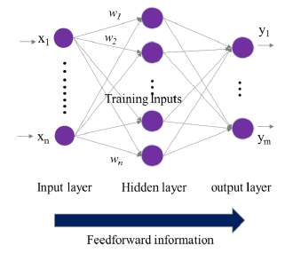
Figure 1: Artificial Neural Network

Since then, the use and application of neural networks have expanded into various fields. In fact, studies have demonstrated that a Multilayer Perceptron network with a single hidden layer has the capability to estimate any function of Rn in Rm with high accuracy [13]. The structure and settings of a neural network are crucial factors that determine its effectiveness and efficiency.The multilayer network is a commonly used structure in neural networks, consisting of an input layer, one or more hidden layers, and an output layer. The hidden layer functions as a mediator between the input and output neurons, and the connections among the layers are represented by the weights of the connecting links. Generally, the layers in a neural network are linked together in a manner that allows data to flow solely in one direction – this is known as a feedforward approach. There are no loops or cycles in the network. The data originates from the input layer, traverses through the hidden layers, and finally arrives at the output layer. An example of a neural network with a single hidden layer is shown in Figure 1 to provide a better understanding of its functioning. In addition, previous research has demonstrated that this architecture is optimal for solving classification problems, which is the focus of this article [13].

For a neural network with one hidden layer, we can observe that each hidden neuron (indexed j = 1,…,n) takes in an input that is the result of a weighted sum of the inputs to the entire network. The transfer function f is used to process the input and convert it into an output signal.

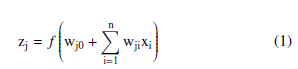
The variable n and and the variable m are the number of input neurons and the hidden ones, respectively and w_ij is the weight from the i_th input neuron to the j_th hidden neuron, x_i is input variable i and w_j0 is a bias term. The hidden neuron signals are subsequently transmitted to the output neurons through weighted connections, similar to the transmission between the input and hidden layers. Consequently, the output neurons obtain the sum of all weighted hidden neurons, which is then passed through a transfer function g, based on the required output range. The output y_o of the network’s output neuron o is formulated as:

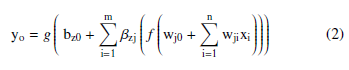
With b_zj represent the weight from the J_TH hidden neuron to the O_th output neuron and b_z0 is the bias. As mentioned earlier, the reason why neural networks are popular in different areas is due to their capacity to approximate linear or nonlinear functions. However, the challenge is to determine the optimal topology and weight values of the network that can closely approximate the target function. This task can be thought of as an optimization problem, where the objective is usually to minimize a cost function based on the total sum of squared errors.

2.4.  Optimizing parameters for ANN

2.4.1     Input variables

Once the artificial neural network is established, the next step is to identify the necessary information required to build the network. This information is provided in the form of input variables that are used to assess the potential job performance of candidates. To permit to the ANN to accurately classify new observations, the input variables must be carefully selected to ensure the classification model performs well. Therefore, it is crucial to identify the most relevant variables for classification purposes.

2.4.2     Architecture

Tthe structure of an ANN is an input layer, output layer, and one or more hidden layers. Hence, there are other crucial factors that have an impact on the performance of the artificial neural network, and they need to be considered while designing it. These factors comprise the number of neurons present in each layer and the number of hidden layers that are incorporated into the network. These parameters determine the behavior of the neural network and vary depending on the problem to be solved.

The study employs the neural network architecture with one hidden layer for classification purposes [13] , which is widely acknowledged as the optimal structure for such problems according to existing literature.

Selecting the appropriate number of neurons for the hidden layers of an artificial neural network can be a difficult task. Having too many neurons can lead to an increase in the number of computations required by the algorithm. Conversely, selecting too few neurons in the hidden layer can result in a reduction in the model’s capacity to learn [14]. So, it is crucial to choose the optimal number of neurons to achieve the highest possible performance of the neural network.

2.4.3     Learning algorithm

The process of finding the optimal weights and biases that maximize the performance of a neural network is known as learning algorithms, which consist of a set of rules. Various techniques have been used in literature to determine the best architectures and topology of weights and biases for the neural network, depending on the learning type.

Supervised learning refers to the scenario where the dataset used for training is labeled, while unsupervised learning train on unlabeled datasets. In unsupervised learning, the weights of the neural network are adjusted based on specific criteria to identify patterns or regularities in the observations.

The principal goal of this research is to improve the performance of an artificial neural network (ANN) in predicting job performance of a candidate. This is done using a supervised learning approach where the labels for the classes are already known and provided during the training stage. The learning algorithm adjusts the connection weights between inputs layers and the target ones to estimate their dependencies and minimize the error function, such as mean squared error.

The optimisation techniques can be classified into two groups: • The first set of techniques is based on the steepest descent method and includes methods like gradient descent, Levenberg Marquardt, Backpropagation, and their variations. However, some of these algorithms require a significant amount of computational resources in terms of time and memory. Out of these, the Backpropagation algorithm is the most widely utilized, as it is a highly effective tool for determining the gradient in neural networks. However, it has its limitations, particularly with regards to the issue of getting stuck in local minima.

• The second group encompasses techniques that are inspired by the evolution of living species, such as genetic algorithms and swarm algorithms among others.

2.4.4     Transfer Function

Before training a neural network, one of the parameters that needs to be determined is the transfer function. The selection of an activation function is dependent on the specific use case. For instance, binary functions are well-suited for organization and distribution problems, whereas continuous and differentiable functions like sigmoid function are utilized to approach continuous functions. Notably, the sigmoid transfer function is commonly used because it combines nearly linear, curvilinear, and nearly constant behavior based on the input value [14]. The sigmoid transfer function’s adaptability enables the artificial neural network to manage both linear and non-linear issues. It’s possible to represent the sigmoid function as:

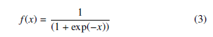
The function being used as the transfer function in this study is bounded between zero and one, and it takes a real-valued input and produces an output within that range.

2.5. Particle Swarm Optimization (PSO)

PSO is an evolutionary computation method that was created by

1. Kennedy, a social psychologist, and R. Eberhart, an electrical engineer, in 1995 [15]. It is a type of swarm intelligence algorithm that draws inspiration from the natural behavior of social organisms, such as birds flocking, and is employed as an optimization technique in a variety of research domains.

Social animals that live in groups, like swarms, often need to travel long distances to migrate or search for food. To do so efficiently, they optimize their movements in terms of time and energy expenditure and cooperate with one another to achieve their objective. The PSO algorithm is rooted in this behavior and is utilized to discover solutions to problems by optimizing a continuous function in a data space. Each member of the group, similar to the animals in a swarm, decides their movement based on their own experience and that of their peers, resulting in a complicated and effective process [15].

The PSO algorithm is designed around a group of individuals known as particles. At the first time, these particles are placed randomly in the solution space and move around in search of the optimal remedy to the challenge. Each particle’s position represents a potential solution to the challenge. The movement of each piece is governed by specific rules. Each particle has a memory that allows it to remember the best point it has encountered so far and tends to return to that point. Additionally, each particle is informed of the best point found by its neighbors and tends to move towards that point.

The initial step for utilizing the PSO algorithm involves establishing a search area comprising of particles and a fitness function for optimization. Afterward, we commence by initializing the system with a set of haphazard solutions (particles). Each particle is allotted a positional value signifying a plausible solution data, a velocity value that denotes the extent to which the data can be modified, and a personal best value (pBest) that represents the particle’s most optimal solution reached thus far.

3. Research Framework

In order to define the solutions, a research framework must first be developed. The research includes four major processes that are included in this research: data collection, preprocessing of data, variable selection, model building and the evaluation of the model.

The proposed framework is shown in the Figure 2 below.

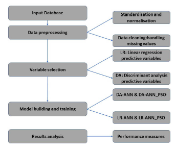
Figure 2: The proposed methodology

3.1. Discriminant variables

To determine the optimal architecture for an ANN, the first step is to identify the input variables. These variables will be used to construct mathematical models that predict job performance. However, selecting the appropriate variables can be a challenge and is crucial for the model’s accuracy. In this study, 15 variables listed in Table 2 were used, based on the availability of data.

3.2. Data preprocessing

Studies and research have demonstrated that several AI algorithms may exhibit poor performance due to the inferior quality of data and variables. Therefore, two critical steps are required to enhance the feasibility of the variables for constructing a predictive model: variable selection modeling for reducing dimensionality and data preprocessing. This process involves data preparation and normalization to accomplish reduction or classification tasks. The Table 1 below shows the variables used in this study.

Table 1: Dataset description

Variables	Description	Value
ID	Employee’s id	integer
Age	Employee’s Age	Integer
Gender	Employee’s gender	M or F
Marital	Employee’s	S or M
status	status
Diploma	Employee Education	Bachelor
	Degree	High Diploma Master, Phd
Experience	Employee	Integer
years	year of experience
Salary	Employee salary	Integer
Communication	Employee level	1 to 5
Level	in communication
Motivation	Employee motivation	Yes or
enthusiasm	for work	No
Language	Employee language	1 to 5
score	level
Specialisation	Employee general	IT, Economics
	Specialisation	HR, Network business
Effectiveness	Employee	Yes or
in a remote	ability	no
environment	in remote
Seniority	Employee seniority	Junior
	in the company	Senior Manager
Physical	Employee ability	Yes or
abilities	to work	no
Additional	Employee additional	Yes or
Certificate	certificate	no
Employee	Employee	BA
performance	performance	Good

3.3. Variables selection models

In classification studies, it is crucial to determine which variables hold the most importance in distinguishing between different categories. Moreover, it is often challenging to obtain trustworthy and meaningful data. Therefore, it is essential to identify the most significant variables that can offer insights to forecast candidate performance to reduce the effort required to gather and verify data.

When creating a prediction model, it can be helpful to reduce the number of variables in order to improve computational efficiency and increase the accuracy of classification algorithms, like neural networks. To achieve this, we’ll use two types of classification techniques statistical methods and artificial intelligence in order to identify the most important variables that distinguish between candidates’ performance. Then, we’ll choose the best variable selection model to optimize the performance of the neural network.

In this study, we are more focused on the statistical method Statistical method used in this study is chosen for its popularity in variable selection is discriminant analysis (DA) and logistic regression. Discriminant analysis is commonly utilized to identify a linear combination of features that can effectively distinguish between two or more groups, in order to reduce the number of dimensions prior to classification.

3.4. Artificial Neural Network Architecture

This study utilizes an ANN model for predicting the job performance of candidates chosen at random. As previously stated, the architecture of the ANN is critical to its functionality and effectiveness. Therefore, this section focuses on determining the optimal topology that can differentiate between a good candidate and a poor one based on the selected variables.

To define the architecture of an ANN, certain parameters must be determined such as the number of input neurons, hidden layers, and hidden neurons. According to the literature, ANNs with one hidden layer are considered the optimal structure for classification problems[13].

4. Cross validation

Any bias or bad quality due to dataset could potentially have a huge impact on determining the artificial neural network and its parameters. In this sense, the cross validation technique is made to minimize this genre of problem.

In our experiment we will use a 3 fold-cross validation technique to train and test our model to avoid over fitting. To be precise, we divided our dataset into three equal subsets, which implies that our model will undergo training and testing procedures three times. The mean value of the accuracy measures obtained from each of the three iterations is used to evaluate the overall accuracy of the model.

5. Performance evaluation

To evaluate the performance of our model, we use this list of evaluation metrics:

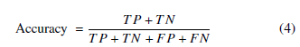
Overall accuracy: In general, accuracy refers to the percentage of correctly classified records by the model. The formula for calculating accuracy can be derived from the confusion matrix presented in Table 2.

Precision: It can be described as the proportion of the correctly predicted cases (True Positive) to the combined number of True Positive and False Positive.

Recall: It can be expressed as the proportion of the correctly predicted cases (True Positive) to the combined number of True Positive and False Negative.

Specificity: The True Negative Rate is calculated as the number of True Negatives divided by the sum of True Negatives and False

Positives.

Predicted
Actual	BA	Good
BA	True Negative	False Positive
Good	False Negative	True Positive

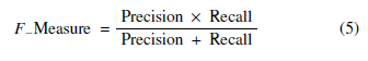
F-Measure: F-measures take the harmonic mean of the Precision and Recall Performance measures [17].

6. Empirical study

As mentioned earlier, the main aim of this study is to employ a combination of neural network and Particle Swarm Optimization to forecast the job performance of a random applicant. The initial stage in this approach, as described in the research methodology, involves choosing the suitable variables that can be utilized to create a the optimal method.

6.1. Data and variables

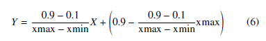
The dataset used in this study issued from a Moroccan firm contains the most variables used on the manual recruitment process based on the survey made inside each department of this firm. Data collected contains more than 1000 individuals. A variable class is created with two values (BA if the candidate is below the average, Good is the candidate have a good qualification). The individuals was selected randomly from a different department: IT department, finance department, HR department, Data department… Before using our Data as input for our model, a normalizing function Eq.6 was applied to bound data values to -1 and +1 with is the input matrix, Y is the normalized matrix, x_min and x_max are respectively the maximal and the minimum values of a variable [18].

6.2.  Results

The initial step of processing and managing data involves dealing with missing values, decreasing the number of variables, and examining the most significant ones, which is crucial. So, we begin our process of building a performance job prediction model by handling the missing values. Our dataset contains many missing values so to fix this problem, we refer to KNN imputation. In fact, a new observation is imputed by finding the samples in the training set closest to it and averages these nearby points to fill in the value.[4]

Secondly, we need to determine the influence of each variables on a candidate’s job performance by using variable selection techniques. We will compare common models such as Discriminant Analysis and Logistic Regression, and summarize the variables selected by each model in a table below.

Table 2: Variables selection results

Variables selection	Number	Selected
Techniques	variables	Variables
		Gender, Marital status, Seniority , Salary
DA	8	Communication level Employee ethics Specialisation, Physical abilities
		Age, Gender, Marital status, Seniority , Salary, Diploma
Logistic		Experience years
Regression	12	Language score Communication score Specialisation, Additional Certificate, Effectiveness in a remote environment

The presented table displays how each model has selected a distinct set of variables based on their discriminatory power. The feature sets have been divided into two categories: the first group contains eight variables chosen by DA, and the second group includes twelve variables chosen by LR.

The ANN model’s input layer will rely on the set of variables selected by the variable selection models. As a result, two hybrid neural network models, MDA-ANN and LR-ANN, are constructed accordingly.

After defining the best variables that will have a big impact on our target variable, it’s time now to define the best architecture for our model, for this reason we compare the following learning algorithm based on PSO, and the hybrid artificial neural network trained separately.

Now, we have reached the step of designing the topology of our hybrid neural network. for this step, we used the following parameters: The architecture that produced the highest performance accuracy applied to our model was determined to be 12-18-1 (12 input neurons, 18 hidden neurons, and one output neuron). The 12 input neurons in this case correspond to the number of variables selected by the logistic regression algorithm, indicating that these variables have strong discriminatory power when it comes to predicting candidate performance.

Table 3: PSO parameters

	Architecture	Weights
Parameters	optimization	optimization
Swarm Size	20	20
Stop criteria & iteration	100	100
Search area range	[3, 20]	[-2.0, 2.0]
Inertia factors	(wn = 0.9 ∗ wn−1)	(wn = 0.9∗ wn−1)
	w0 = 0.8	w0 = 0.8

We can see also that the application of our Hybrid artificial neural network separately decrease the performance of the two models DA-ANN and LR-ANN compared to its application with the PSO. The results will be presented and analyzed in the table 5.

Note that the evaluation of the evaluation metrics alone does not give a good judgment on the quality of the prediction and the classification. In this performance comparison, we will also focus on the performance attribute to each class which gives important information about a model especially to select the variables which discriminate the performance of the candidates.

This appears clearly in the application of the hybrid algorithm: DA-ANN and DA-ANN PSO. In fact, even with its big accuracy, they present the less rate of good classification of good candidates (47.5%, 48.3%) contrary to below average candidates (between 83.3% and 83.4%). The LR-ANN PSO model gives the best classification rate. These findings suggest that the variables identified by the LR statistical models provide more insights into a candidate’s job performance.

Table 4: Results

Model	LR-ANN	LR-ANN PSO	DA-ANN	DA-ANN
Accuracy	72.5%	75.0%	65.0%	65.4%
Precision	70.1%	72.9%	47.5%	48.3%
Sensitivity	73.1%	75.6%	74.9%	75.1%
Specificity	72.0%	74.5%	60.3%	60.6%
F-measure	71.6%	74.2%	58.1%	58.8%
BA	74.9%	77.0%	83.4%	83,3%
Good	70.1%	72.9%	47.5%	48.3%

7. Conclusion

In this research, we have implemented a hybrid discriminant neural network relying on particle swarm optimisation and statistical variables selection techniques. The models developed takes into account the variables mostly used in the manuel performance job prediction, otherwise, the constraints of missing values was fixed by the K-nearest neighbor algorithm.

The proposed methodology of variables selection evaluated the impact of different variables selection models by comparing Multivariate Discriminant Analysis and Logistic Regression. The findings demonstrate that logistic regression perform exceptionally well as a variables selection model for Artificial Neural Networks (ANN) to distinguish between candidates job performance. Moreover, the application of the variables chosen by this technique gives the best performance for the task of prediction the candidate job performance prediction.

The hybrid neural network applied with the learning algorithm PSO gives the best results in term of optimisation and finding the local minima and then in the prediction of the job performance. This model will be very useful for recruiter to assess and predict the performance of future candidates.

1. S. S. A. Mohan, Support Vector Machines for Job Performance Prediction: A Comparative Study, Ph.D. thesis, 2021.
2. J. Zhang, Y. Liu, The Use of Big Data Analytics in Job Performance Prediction: A Literature Review, Ph.D. thesis, 2020.
3. S. Kaur, M. Singh., “A Review of Machine Learning Algorithms for Job Performance Prediction,” 2019.
4. J. Delaney, The rise of predictive employee analytics, Ph.D. thesis, 2019.
5. S. Krishnan, Predictive employee analytics: A new frontier in HR. Forbes., Ph.D. thesis, 2020.
6. D. L. . C. J.Russell, Employee analytics: How to improve business performance by measuring and managing your workforce., Ph.D. thesis, 2015.
7. H. . Y.Zhang, A review of predictive analytics in human resources management., Ph.D. thesis, 2018.
8. J. Han, M. Kamber, Data Mining: Concepts and Techniques, Ph.D. thesis, 2006.
9. K. K. Y. Geoffrey K.F. Tso, “Predicting electricity energy consumption: A comparison of regression analysis, decision tree and neural networks,” Energy, 32, 1761–1768, 2007, doi:doi.org/10.1016/j.energy.2006.11.010.
10. E. D. et P. Na¨ım, Des re´seaux de Neurones, EYROLLES, 1992.
11. F. Rosenblatt, “The perceptron: a probabilistic model for information storage and organization in the brain.” Journal of Applied Mathematics and Physics, 5, 1958, doi:doi.org/10.1037/h0042519.
12. J. L. M. David E. Rumelhart, “Parallel distributed processing: explorations in the microstructure of cognition, vol. 1 : foundations,” The MIT Press, 9, 386–408, 1987.
13. Y.-C. L. Jae H. Min a, “Bankruptcy prediction using support vector machine with optimal choice of kernel function parameters,” Expert Systems with Ap- plications, 28, 603–614, 2005, doi:doi.org/10.1016/j.eswa.2004.12.008.
14. D. T. L. et C. D. Laros, Discovering Knowledge in Data: An Introduction to Data Mining, Second Edition, WILEY, 2014.
15. J. K. R. Eberhart, “A new optimizer using particle swarm theory,” MHS’95. Proceedings of the Sixth International Symposium on Micro Machine and Human Science, doi:10.1109/MHS.1995.494215.
16. S. A. Fatima Zahra Azayite, “Topology design of bankruptcy prediction neural networks using Particle swarm optimization and backpropagation,” 1–6, 2018, doi:https://doi.org/10.1145/3230905.3230951.
17. “Archives ourvertes,” 2018.
18. “cyberleninka,” 2018.

(Click Here)