1. Introduction

This paper is an extension of work initially presented at the 2022 IEEE Symposium on Computer Applications & Industrial Electronics (ISCAIE2022)[1]. Planning and estimation are imperative for any Information Technology (IT) project. Estimation aids in tracking progress and delivery velocity. However, due to the close relationship between cost and time factors, any project delay might result in cost overruns.

The investigators [2][3] revealed that the top-ranked IT project risk is “Underestimated Costs and Time”. According to the authors [4], 60% of IT projects have cost and time problems. Budget and timeline underestimation seems to occur at various stages of the project lifecycle. The most undesirable scenario happens when the budget and duration are underestimated at the beginning of the project lifecycle.

Artificial intelligence (AI) can improve decision-making in complex environments with clear objectives. A study concluded that, in terms of accuracy, artificial intelligence tools outperform traditional tools [5]. The value of AI can only be activated as humans and machines function complementarily integrated.

Hybridizing Machine Learning (ML) models are getting their popularity recently. According to researchers [6], hybridization effectively advances prediction models. This article focuses on the performance of various hybrid ML models in prediction accuracy enhancement to improve cost and duration estimation to address the critical IT failure problem.

2. Methodology

2.1.  The Machine Learning Model Evaluation

This study was designed to demonstrate to the research community that the evaluations are comprehensive and can explain their significance. Five hybrid ML models were developed using Python and evaluated using three different datasets, including two public datasets. These models were trained and tested on three different datasets to reduce bias caused by data quality. The best-performing ML model was selected based on the performance measured by six different metrics. It was then put forward for live project verification to determine its performance in predicting project cost and duration.

These five hybrid ML models were: Hybrid Multiple Linear Regression Deep Neural Network (MLR-DNN), Particle Swarm Optimised DNN (PSO-DNN), Hybrid Gradient Boosting Regression DNN (GBR-DNN), Hybrid Random Forest Regression DNN (RFR-DNN), and Hybrid eXtreme Gradient Boosting DNN (XGB-DNN).

Controlled experiments play a vital role in applied machine learning, and the behaviour of algorithms on specific problems must be learned empirically. A machine learning experiment procedure involves a series of steps, 1. Data collection. 2. Data pre-processing: cleaning and manipulating acquired data to prepare it for modelling. 3. Model training: the model is trained on a training dataset, usually a subset of the data collected. 4. Model tuning: change in hyperparameters to optimize the model’s performance. ML performance is measured by the defined performance metrics indicated in section 2.2.  5. Model evaluation: determine the model’s performance on a testing dataset or another subset of the data collected. 6. Model deployment: the best model is then used to make predictions on live project data.

2.2.  Performance Metrics

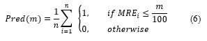
Evaluating the performance of ML models is essential to ensure their effectiveness. The choice of the performance metric is an important factor in this evaluation process. It depends on the specific ML problem being solved and the project’s goals. The performance parameter used in this study is accuracy, which evaluates the number of correct predictions made as a percentage of all predictions made. The associated “accuracy” performance metrics used were , , , ,  and ( ).

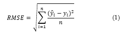
The Root Mean Square Error ( ) acts as a heuristic model for testing and training measures differences between predicted values and actual values from 0 to ∞. The smaller the , the better the model [7].   is predicted output or forecasted values and  is the actual or observational values.

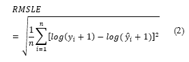
The Root Mean Squared Log Error ( ) is a logarithmically calculated  commonly used metric or loss function in the regression-based machine learning model. The lesser error, the better the model is.

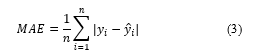
The Mean Absolute Error ( )  measures the magnitude of errors regardless of their direction in a series of estimates.  is superior to  in terms of explanation-ability.  has a distinct advantage over  using absolute values, which is undesirable in many mathematical calculations. The smaller value, the better the model is.

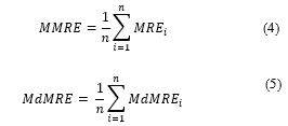
The Mean Magnitude of Relative Error ( ) and Median Magnitude of Relative Error ( ) are two important performance metrics derived from the overall mean and median errors. The primary function of  is to serve as an indicator for differentiating between prediction models. The model with the lowest  typically being chosen typically implies low uncertainty or inaccuracy. The better the model, the smaller the values are.

Percentage of Estimate, , is an alternative to the  that is a commonly used prediction quality metric. It simply measures the proportion of forecasts within % the actual value. The bigger the , the less information and confidence in a prediction’s accuracy [8].

2.3.  Degree of Augmentation

The degree of augmentation (DOA), , is a prediction enhancement measurement in error reduction to measure a hybrid model. A dual-layer hybrid cascaded ML model comprises two ML models represented as layers one and two (Figure 1). In stage one, the layer one ML model makes a prediction value  as inputs to stage two ( ) to be processed by the layer two ML model with prediction output . The difference (or error) in the predicted result versus the actual result at stage one is denoted as .

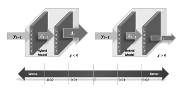
Figure 1: The Degree of Augmentation Scale

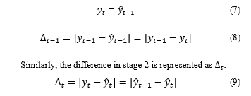
The assumption of difference in stage two is more diminutive than in stage one. The effect of convergence resulted in  reduction; therefore, augmentation occurred.

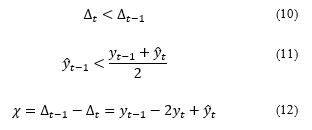
By using equation (12), the  for stage one ( ) and stage two ( ) enables to calculate of the degree of augmentation, , for each of the hybrid models. The degree of augmentation,  is bi-directional. A negative value indicates  increases or diverging, whereas a positive value specifies  decrease or converges. The positive magnitude of  shows the strength of augmentation. The higher the  means the better the hybrid model. The more significant negative value of  means the hybrid model is ineffective.  is considered effective,  is ineffective. For   is marginally effective, which means its augmentation is not significant enough to remain effective.

In an optimistic augmentation scenario, the Interquartile Range (IQR) becomes narrower, whereas the range becomes wider in an adverse augmentation scenario. This convergent phenomenon indicates the  decreases in positive augmentation. Contrary, in a divergent case,  increases in negative boost.

2.4.  Data Collection

Figure 2 illustrates the data collection procedure. Each dataset was randomly split into two groups in a 70:30 ratio, 70% for training and 30% for testing. The relevant dataset was acquired online or gathered from previous project material. The collected data was then converted (if necessary) and pre-processed using scaling (for example, the scikit-learn scaling package) to prepare for ML assessment.

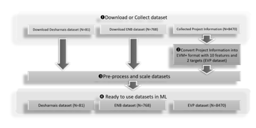
Figure 2: The data collection procedure

2.5.  ML Evaluation

These ML models were evaluated in three steps depending on their algorithm settings. First, the respective models were trained using historical data in the learning or training step. Later in the testing step, these ML models were tested based on a peer comparison of their performance indicators. Each ML model was optimized through hyperparameter tuning until the best results were obtained (Figure 3).

2.6.  Dataset Descriptions

A study concurs that the model may poorly correlate with a dataset that makes learning “incomplete” [9]. This evaluation used three dataset sources to minimize potential bias due to the dataset’s influences. Two are publicly available, and the third dataset is a collection of actual historical project data named EVP. Both Desharnais and ENB datasets were selected in this study because of their multi-target attributes.

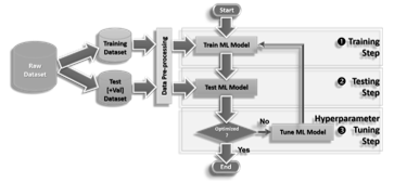
Figure 3: The ML evaluation workflow

It is challenging to ensure the quality of an ML dataset, mainly because the relationship between the qualities of the data and their effect on the ML system’s compliance with its requirements is infamously complex and hard to establish [10]. In this study, dataset quality was defined as its appropriateness in terms of accuracy and value.

1)       Desharnais Dataset

Jean-Marc Desharnais gathered the Desharnais dataset from ten organizations in Canada between 1983 and 1988. There are 81 projects (records) and 12 attributes [11], a relatively small public dataset of which four nominal fields are considered redundant in ML model evaluation. Table 1 provides statistical information about this dataset. Four entries have missing data. Most studies that use this dataset use 77 of the 81 records [12]. This study backfilled the missing fields with a “-1” value. Small dataset size issues could be compensated by adopting data-efficient learning or data augmentation strategies [13]. Desharnais datasets were used in many research. Therefore, it can benchmark the investigation against other published results.

2)       ENB Dataset

The Energy Building Dataset [14] contains 768 instances of eight measured building parameters as feature variables. The dataset includes the two corresponding target heating load and cooling load attributes. A nominal field is considered redundant in this dataset.

Table 2 provides statistical information about this public dataset. The data comes from real-world applications and reflects real-world events with a multi-target. ENB is another popular dataset being used by many studies. The data size is deemed appropriate with more than 300 samples [15]. The ENB dataset is interesting, with only two targets closely associated, while the features have no interdependency, making prediction more complicated.

Table 1: Descriptive Statistics for Desharnais Dataset

Descriptive Statistics	id	Proj	Team Exp	Mgr Exp	Year End	LEN	Effort	TRXN	Entities	Points Non Adjust	Adjust	Points Adjust	LANG
Valid	81	81	81	81	81	81	81	81	81	81	81	81	81
Missing	0	0	0	0	0	0	0	0	0	0	0	0	0
Mean	41.00	41.00	2.19	2.53	85.74	11.67	5046.31	182.12	122.33	304.46	27.63	289.23	1.56
Std. Deviation	23.53	23.53	1.42	1.64	1.22	7.43	4418.77	144.04	84.88	180.21	10.59	185.76	.71
IQR	40.00	40.00	3.00	3.00	2.00	8.00	3570.00	136.00	112.00	208.00	15.00	199.00	1.00
Minimum	1.00	1.00	-1.00	-1.00	82.00	1.00	546.00	9.00	7.00	73.00	5.00	62.00	1.00
Maximum	81.00	81.00	4.00	7.00	88.00	39.00	23940.00	886.00	387.00	1127.00	52.00	1116.00	3.00

Table 2: Descriptive Statistics for ENB Dataset

Descriptive Statistics	id	Relative compactness	X1	X3	X4	X5	X6	X7	X8	Y1	Y2
Valid	768	768	768	768	768	768	768	768	768	768	768
Missing	0	0	0	0	0	0	0	0	0	0	0
Mean	384.500	.764	671.708	318.500	176.604	5.250	3.500	.234	2.813	22.307	24.588
Std. Deviation	221.847	.106	88.086	43.626	45.166	1.751	1.119	.133	1.551	10.090	9.513
IQR	383.500	.147	134.750	49.000	79.625	3.500	1.500	.300	2.250	18.675	17.513
Minimum	1.000	.620	514.500	245.000	110.250	3.500	2.000	.000	.000	6.010	10.900
Maximum	768.000	.980	808.500	416.500	220.500	7.000	5.000	.400	5.000	43.100	48.030

Table 3: Descriptive Statistics for EVP Dataset

Descriptive Statistics	X1	X2	X3	X4	X5	X6	X7	X8	X9	X10	Y1	Y2
Valid	8470	8470	8470	8470	8470	8470	8470	8470	8470	8470	8470	8470
Missing	0	0	0	0	0	0	0	0	0	0	0	0
Mean	.500	.053	.642	.633	.804	.791	3.057	1.162	.170	.013	1.002	.838
Std. Deviation	.006	.139	.276	.318	.272	.318	18.152	2.354	.316	.203	.205	.251
IQR	.000	.035	.446	.554	.297	.314	.926	.079	.375	.059	.042	.245
Minimum (x10-3)	.500	141.9	3.000	34.55	8.000	7.000	460.0	99.00	-1524	-3953	.000	35.15
Maximum	1.000	1.000	1.611	3.976	3.774	4.757	1461.738	136.935	2.864	1.068	4.700	2.656

3)       EVP Dataset

Earned Value Management (EVM) is widely acknowledged as the most reliable contemporary project management instrument or cost and timeline forecasting technique. EVM calculates the amount of work performed to measure project performance and progress. The Earned Value Plus dataset is based on the conventional EVM attributes and added two new attributes related to the project management and size indexes. It contains 8,470 (more than 8000 records) instances from more than 600 historical project data in EVM format was deemed sufficient to train the ML model effectively (Table 3).

3. Experimental Results

Each optimized model was tested in four cycles. Evaluation results were obtained through each testing cycle and tabulated for each performance indicator. Each performance metric was calculated based on the average performance. The following subsections describe how the ML model performed, illustrated by graphical presentation in two graphs. The first graph shows performance results in ,  and . The second graph shows the performance results in ,  and .

3.1.  Desharnais Dataset

MLR-DNN was the most optimal model for predicting the probability of a given experiment, while PSO-DNN appeared as the worst. MLR-NNN had the highest  value and the best  and  values among all models tested in this study (Figure 4 and Figure 5). MLR-DNN is a hybrid cascaded ML model comprising MLR (Multiple Linear Regressor) and cascading with DNN (Deep Neural Network) embedded with four hidden layers and 64 neurons in each hidden layer.

Figure 4: The , , and  results in the Desharnais dataset

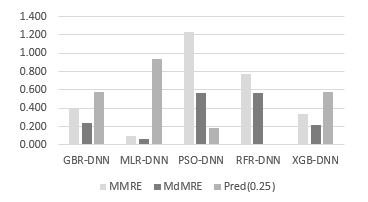
Figure 5: The , , (25) results in the Desharnais dataset

3.2.  ENB Dataset

MLR-DNN outplayed all other performance metrics, with the lowest  value being the least desirable model. The optimum  value was .011, and the highest  value was .492, according to the most favourable  value. The most accurate  value was .004 (Figure 6 and Figure 7).

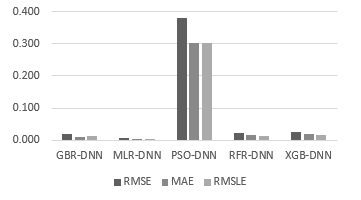
Figure 6: The , , and  results in the ENB dataset

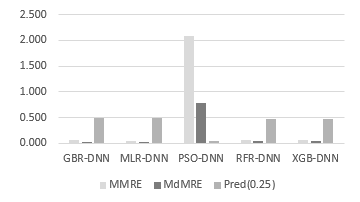
Figure 7: The , , (25) results in the ENB dataset

3.3.  EVP Dataset

MLR-DNN ranked as the top-performing ML model, with the lowest  value and highest  value. The most favourable  value was .003, the best  value was .003 and the most accurate  value of <.001 (Figure 8 and Figure 9).

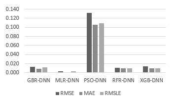
Figure 8: The , , and  results in the EVP dataset

3.4.  Degree of Augmentation

The degree of augmentation, , is used as an error reduction indicator in a cascaded hybrid ML model using equation (12). The  for stage one ( ) and stage two ( ) enables us to calculate the degree of augmentation,  , for each of the hybrids cascaded ML models (Figure 1). The hybrid model MLR-DNN demonstrated an average error reduction of .026 compared to the MLR model alone. PSO-DNN was excluded from the DOA comparison because PSD-DNN is not a cascaded standalone ML model but part of DNN with Particle Swarm Optimization (PSO) backpropagation. Overall results revealed that MLR-DNN outperformed all three other hybrids cascading DNN models, suggesting that cascading two different ML models may not produce positive results. Both GBR-DNN and XGB-DNN did not improve prediction accuracy, whereas the RFR-DNN model performed worse than RFR or DNN alone.

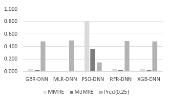
Figure 9: The , , (25) results in the EVP dataset

Based on the performance results, the MLR-DNN model performed exceptionally well on all three datasets. The dependency on the quality of the dataset remains significant. This finding indicated that the PSO-DNN model was the most underwhelming performer in ENB and EVP datasets. However, for all three datasets, the least compelling performer was PSO-DNN. The runner-up position for both ENB and EVP datasets was GBR-DNN. However, the runner-up for the Dasharnais dataset was XGB-DNN.

The results also indicated that hybrid cascaded ML models such as GBR-DNN & XGB-DNN do not guarantee a positive gain and may sometimes have detrimental effects, for example, the RFR-DNN model. GBR-DNN performed relatively well in Desharnais and ENB datasets. However, it performed poorly in the EVP dataset. The result indicated that the quality of the dataset remains significant. This finding opens the door for future research.

The interquartile range ( ) is a reliable measure of variability representing the dispersion of the middle 50% of the data [16]. The  is calculated as  = Q3 − Q1 statistically; the smaller  indicates the error range is relatively small. MLR-DNN showed the narrowest  and largest Mann-Whitney U effect size to strengthen its position as the most accurate ML model among the other models in this study. MLR-DNN enhanced the overall prediction accuracy compared to other models with a significant magnitude of error reduction.

From observation of the statistical value in Table 4 for the degree of augmentation   and Mann-Whitney U test effect size , it seems like there is some form of proportion. The investigators [17] explained that effect size is the difference between the variable’s value in the control and test groups. The magnitude of  increases and  increases, . The significant difference between  and  is that the effect size does not cater to attributes of positive or negative augmentation. This finding reflects that the degree of augmentation is a more appropriate performance indicator for measuring cascaded hybrid ML models.

Table 4: Degree of Augmentation Statistical Data

	GBR-DNN		MLR-DNN		RFR-DNN		XGB-DNN
Descriptive statistics
Valid	11857	1779	11857	1779	11857	1779	11857	1779
Missing	0	0	0	0	0	0	0	0
Mean	.007	.006	.028	.002	.006	.009	.006	.006
Std. Deviation	.019	.018	.035	.003	.018	.011	.018	.014
	.006	.006	.024	.001	.005	.007	.005	.005
Minimum (x10-6)	.105	8.492	12.13	1.059	.001	51.88	.002	.083
Maximum	.615	.115	.578	.061	.648	.188	.659	.397
-value of Shapiro-Wilk		<.001		<.001		<.001		<.001
Degree of Augmentation		.001		.026		-.003		.000
Mann-Whitney		9205868		809668		6171934.5		8978979
Wilcoxon		79517879		2394758		76472087.5		79290990
( ) score		-8.701		-62.910		-28.286		-10.166
-value		.000		.000		.000		.000
Effect Size r		.074		.538		.239		.061

4. Verification Results

Three types of live project data (Waterfall, Hybrid, and Agile) were used to verify MLR-DNN performance. The live performance results explained how effective MLR-DNN could be used practically in project management.

4.1.  Waterfall Project

XYZ is one of the largest telecommunications operators in South East Asia. Due to exponential growth in customer demand, XYZ decided to enhance its operations support capability. MLR-DNN was used during the live project verification stage to forecast the budget and duration. Two EVM data samples were collected at 43% and 53% completion points. Table 5 displays the results.

MLR-DNN outperformed traditional EVM by 8.4% and 54.1% in average cost at Estimate At Completion (EAC) and average schedule prediction at Estimate Duration At Completion (EDAC), respectively. These findings align with a study which indicates CPI (cost) accuracy is relatively better than SPI (time) accuracy in EVM calculation [18].

Table 5: Waterfall Project Verification

% Complete	Actual		ML Prediction
	EAC	EDAC	EAC	EDAC	EAC	EDAC
43%	.70	.67	.80	.65	.1	.02
53%	.70	.67	.74	.65	.04	.02
					.07	.02

The MLR-DNN model improved and significantly enhanced the performance of project effort and duration estimation. Work Breakdown Structure (WBS) and EVM remain moderately accurate despite being less dependent on humans. The result indicated that the dataset’s quality continues to have a significant impact, opening future research opportunities.

4.2.  Hybrid Waterfall-Agile Project

Hybrid Agile-Waterfall projects combine agile approaches with waterfall methodologies to deliver projects. The waterfall method to record specific requirements and the agile methodology to deliver gradually in sprints are examples of hybrid projects. Another hybrid agile-waterfall model is software development teams adopting the agile methodology, while hardware implementation teams stick to the waterfall approach. The amount of agile versus waterfall project technique adoption in scope coverage determines the blending ratio.

STU is a major telecommunications operator in South East Asia with millions of customers. It would like to optimize and enhance its operations support and telemarketing capability. The project cost is moderately high: hardware, commercial out-of-shelf products, software customization, system integration, consulting, and professional services.

Table 6: Hybrid Waterfall-Agile Project Verification

% Complete	Actual		ML Prediction
	EAC	EDAC	EAC	EDAC	EAC	EDAC
31%	.86	.96	1.23	.82	.37	.14
38%	.86	.96	.88	.73	.02	.23
54%	.86	.96	.84	.81	.02	.15
70%	.86	.96	.88	.74	.02	.22
92%	.86	.96	.75	.92	.11	.04
					.11	.16

Five samples were collected from the same project at different stages and times (Table 6). One noticeable phenomenon is that prediction accuracy depends on the percentage of completion points. The closer the project’s end, the more accurate the forecast is. At 31% completion, it was a less accurate prediction than the 54% completion point. The characteristic of EVM is inherited and aligned with findings shared by Urgilés et al. [10].

The predicted EDAC was accurate enough, with an average variance of 16% compared to any existing PM techniques and tools with 35-60%. There were insufficient details as to why there was a higher variance of EDAC than compared to EAC. Nevertheless, the project details revealed many change requests initiated that might impact prediction accuracy.

4.3.  Agile Project

The MLR-DNN was fed with live agile project-scaled EVP data to predict project duration and cost in this verification test. Agile projects are typically shorter in duration and use fixed-length iterations. These projects usually have a low to medium budget, fixed period, and flexible scope.

ABC is a popular online banking software offering various electronic payment services to customers and financial institutions. A backlog of enhancements was prioritized in a different sprint by adopting a 100% agile methodology for the whole software development life cycle. Project resources were relatively small, usually less than ten people.

Project size was determined by the amount of project value in USD. Project is considered “small” < 500k; 1 million > “medium” ≥ 500k, and “large” > 1 million. The percentage of completion was defined as the average project delivery progress

Table 7: Agile Project Verification

% Complete	Actual		ML Prediction
	EAC	EDAC	EAC	EDAC	EAC	EDAC
100% (Sprint 1)	1	1	.99	1.00	.01	0
100% (Sprint 2)	1	1	.99	.99	.01	.01
50% (Sprint 3)	1	1	.77	.59	.23	.41
70% (Sprint 4)	.85	1	.93	.77	.08	.23
80% (Sprint 5)	.92	1	.94	.86	.02	.14
					.07	.16

Three project-type live data samples were collected at different stages, iterations, sprints, and releases comprised of Agile, Hybrid, and Waterfall projects (Table 7). The overall prediction accuracy comparison between traditional EVM vs MLR-DNN in three project types is illustrated in Figure 10.

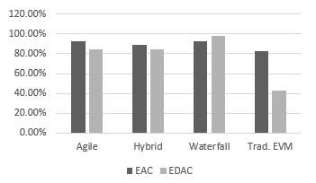
Figure 10: Performance Comparison between MLR-DNN and Traditional EVM in both Schedule and Cost Prediction

MLR-DNN model performed well in agile projects. It accurately predicted cost and schedule dimensions for many waterfall projects. Cost forecast accuracy is relatively better than duration forecast accuracy.

5. Machine Learning Biases

Machine learning (ML) algorithms are becoming more used in various industries. These algorithms, however, are not immune to bias, which can have detrimental repercussions. Therefore, it is critical to understand and address potential ML biases in order to ensure that these algorithms are fair and equal.

Type I – Algorithmic bias refers to systematic errors or unfairness resulting from employing algorithms inherited from the ML model, including how the model was constructed or trained, leading to biased outcomes [19]. Type II – Dataset bias is another type of bias that relates to the tendency of ML models to deliver inaccurate or unreliable predictions due to flaws or inconsistencies in the data used to train them [20]. It can result from various factors, including data collection methods and pre-processing techniques. To reduce ML biases, practitioners should evaluate models and datasets for performance and choose the least biased models.

6. Conclusion and Further Research

Traditional project planning in effort and duration estimation techniques remain low to medium accurate. This study seeks to develop a highly reliable and efficient Hybrid ML model that can improve cost and duration prediction accuracy. The results of the experiments indicated that MLR-DNN was the superior, effective, and reliable machine learning model.

The verification results in Agile, Hybrid and Waterfall projects indicated that the MLR-DNN model improved and significantly enhanced project effort performance and duration estimation. Despite WBS and EVM (conventional project management tools) being less dependent on humans, they are moderately accurate.

The results indicated that hybrid cascaded ML models such as GBR-DNN & XBG-DNN do not guarantee a positive gain and may sometimes have detrimental effects, for example, the RFR-DNN model. MLR-DNN inherits other neural network flaws being computationally costly and operating in black boxes with little explanation.

The accuracy of neural networks (including MLR-DNN) depends on the volume and the quality of training data [21]. Therefore, the dataset’s quality significantly impacts the ML model’s performance. This finding opens the door for future research.

1. D.-J. Pang, K. Shavarebi, S. Ng, “Development of Machine Learning Models for Prediction of IT project Cost and Duration,” in 2022 IEEE 12th Symposium on Computer Applications & Industrial Electronics (ISCAIE), IEEE: 228–232, 2022, doi:10.1109/ISCAIE54458.2022.9794529.
2. D.-J. Pang, K. Shavarebi, S. Ng, “Project practitioner experience in risk ranking analysis-an empirical study in Malaysia and Singapore,” Operations Research and Decisions, 32(2), 2022, doi:10.37190/ord220208.
3. D.-J. Pang, K. Shavarebi, S. Ng, “Project Risk Ranking Based on Principal Component Analysis – An Empirical Study in Malaysia-Singapore Context,” International Journal of Innovative Computing, Information and Control, 18(06), 1857–1870, 2022, doi:10.24507/IJICIC.18.06.1857.
4. TD. Nguyen, T.M. Nguyen, T.H. Cao, “A conceptual framework for is project success,” in Lecture Notes of the Institute for Computer Sciences, Social-Informatics and Telecommunications Engineering, LNICST, 142–154, 2017, doi:10.1007/978-3-319-56357-2_15.
5. D. Magaña Martínez, J.C. Fernandez-Rodriguez, “Artificial Intelligence Applied to Project Success: A Literature Review,” International Journal of Interactive Multimedia and Artificial Intelligence, 3(5), 77, 2015, doi:10.9781/ijimai.2015.3510.
6. A. Mosavi, M. Salimi, S.F. Ardabili, T. Rabczuk, S. Shamshirband, A.R. Varkonyi-Koczy, “State of the art of machine learning models in energy systems, a systematic review,” Mdpi.Com, 12(7), 2019, doi:10.3390/en12071301.
7. S. Bayram, S. Al-Jibouri, “Efficacy of Estimation Methods in Forecasting Building Projects’ Costs,” Journal of Construction Engineering and Management, 142(11), 05016012, 2016, doi:10.1061/(ASCE)CO.1943-7862.0001183.
8. D. Port, M. Korte, “Comparative studies of the model evaluation criterions MMRE and PRED in software cost estimation research,” in ESEM’08: Proceedings of the 2008 ACM-IEEE International Symposium on Empirical Software Engineering and Measurement, ACM Press, New York, New York, USA: 51–60, 2008, doi:10.1145/1414004.1414015.
9. E. Korneva, H. Blockeel, “Towards Better Evaluation of Multi-target Regression Models,” in Communications in Computer and Information Science, Springer Science and Business Media Deutschland GmbH: 353–362, 2020, doi:10.1007/978-3-030-65965-3_23.
10. S. Picard, C. Chapdelaine, C. Cappi, L. Gardes, E. Jenn, B. Lefevre, T. Soumarmon, “Ensuring Dataset Quality for Machine Learning Certification,” in Proceedings – 2020 IEEE 31st International Symposium on Software Reliability Engineering Workshops, ISSREW 2020, 275–282, 2020, doi:10.1109/ISSREW51248.2020.00085.
11. A.K. Bardsiri, “An intelligent model to predict the development time and budget of software projects,” International Journal of Nonlinear Analysis and Applications, 11(2), 85–102, 2020, doi:10.22075/ijnaa.2020.4384.
12. MF Bosu, SG Macdonell, “Experience: Quality benchmarking of datasets used in software effort estimation,” Journal of Data and Information Quality, 11(4), 1–26, 2019, doi:10.1145/3328746.
13. R.M. Thomas, W. Bruin, P. Zhutovsky, G. Van Wingen, “Dealing with missing data, small sample sizes, and heterogeneity in machine learning studies of brain disorders,” Machine Learning, 249–266, 2019, doi:10.1016/B978-0-12-815739-8.00014-6.
14. OpenML enb, May 2021.
15. M.A. Bujang, N. Sa’at, T.M. Ikhwan, T.A.B. Sidik, “Determination of Minimum Sample Size Requirement for Multiple Linear Regression and Analysis of Covariance Based on Experimental and Non-experimental Studies,” Epidemiology Biostatistics and Public Health, 14(3), e12117-1 to e12117-9, 2017, doi:10.2427/12117.
16. D.T. Larose, Discovering Knowledge in Data: An Introduction to Data Mining, 2005, doi:10.1002/0471687545.
17. P. Kadam, S. Bhalerao, “Sample size calculation,” International Journal of Ayurveda Research, 1(1), 55, 2010, doi:10.4103/0974-7788.59946.
18. M. Fasanghari, S.H. Iranmanesh, M.S. Amalnick, “Predicting the success of projects using evolutionary hybrid fuzzy neural network method in early stages,” Journal of Multiple-Valued Logic and Soft Computing, 25(2–3), 291–321, 2015.
19. S.S. Gervasi, I.Y. Chen, A. Smith-Mclallen, D. Sontag, Z. Obermeyer, M. Vennera, R. Chawla, “The Potential For Bias In Machine Learning And Opportunities For Health Insurers To Address It,” Https://Doi.Org/10.1377/Hlthaff.2021.01287, 41(2), 212–218, 2022, doi:10.1377/HLTHAFF.2021.01287.
20. A. Paullada, I.D. Raji, E.M. Bender, E. Denton, A. Hanna, “Data and its (dis)contents: A survey of dataset development and use in machine learning research,” Patterns, 2(11), 100336, 2021, doi:10.1016/J.PATTER.2021.100336.
21. J. Zhou, X. Li, H.S. Mitri, “Classification of rockburst in underground projects: Comparison of ten supervised learning methods,” Journal of Computing in Civil Engineering, 30(5), 04016003, 2016, doi:10.1061/(ASCE)CP.1943-5487.0000553.

(Click Here)