1. Introduction

Solar energy is the bedrock of alternative energy sources since it may be used to develop other renewable energies [1]. In addition, photochemical power operations and other physical processes both heavily rely on solar energy. The earth’s surface will receive solar energy via a radiation mechanism. The radiation will be filtered into the atmospheric layer, which contains gaseous substances as well as other solid forms including water vapour, dust, and aerosols, before it reaches the surface of the planet [2]. This filtration procedure has lowered the solar radiation’s intensity to the point where it will not damage earthly life. The geographic position of a region on the earth’s surface affects the amount of solar energy that reaches that region [3]. As a result, there are three ways to gather information about the intensity of solar radiation in a given area: directly using pyranometers, pyrheliometers, and Campbell Stokest measuring instruments; using satellite image data; and numerical simulation through computer modeling to determine the potential for future radiation. However, due to a lack of measuring tools, there is still extremely little and difficult-to-access sun irradiation data available in Indonesia. Since satellite image data is internationally available, it is widely used [4].

The escalation of world energy demand and the need for environmentally sustainable development have attracted human attention to renewable energy sources [5]. Among the renewable energy sources, solar power has become increasingly prevalent as a utility-scale renewable energy supply due to its simplicity of installation and maintenance.  Furthermore, solar technology has matured, and mass manufacturing of PV panels as the core component of a solar power plant has reduced the cost. Thus, solar power integration into the grid is on the rise, and facilities might be present in the coming years [6].

Power losses in an electric power grid are caused by the current flowing in the conductor lines, where long conductor lines with large loads will result in significant power losses. However, this power loss cannot be avoided, so the only thing that can be done is to minimize the loss. Some of the methods that have been offered in previous research to minimize the losses include power injection through flexible alternating current transmission systems (FACTS) [7,8], distributed generators (DGs) [9–13],  and optimal sizing and placement of capacitors [14–16], so that the voltage profile can be corrected, which results in minimal power losses.

In this paper, a model for forecasting solar irradiation was created for use in the Manokwari region and its surrounds, which are located at latitude -0.8457 and longitude 134.0504. The model was created using an extreme learning machine (ELM) algorithm that is modified from a neural network to improve learning speed. The model is used to forecast the local daily solar irradiation intensity. The data is then used to calculate the potency for minimizing power losses through the interconnection of a 1 MWp solar power plant to an existing power grid around the location. Then the objectives of this paper are given as: 1) designing a suitable model for the specific area based on the ELM algorithm, 2) forecasting the day-ahead solar irradiance for that location, and 3) investigating the possibility of power loss minimization in a power grid based on the forecasting data. This paper is an extension of work originally presented at the CyberneticsCom conference [1].

The frame of the paper is structured as follows: Section II  provides problem statement. Section III describes the research approach and the methods used. The data source, results, and explanations of the findings are presented in Section IV. The paper’s primary research findings are summarized in Section V.

2. Problem Statement

Previous research on power losses has been argued in [17],  who have developed the Power Voltage Sensitivity Constant (PVSC), which has been developed to determine the location and size of multiple DG units so that active power losses in a distribution system can be reduced. The method was tested on an IEEE 69 reconfigured bus system under three different total loads and heavy conditions. It can be concluded from the results that the proposed methodology gives maximum loss reduction while considering DG size. Authors in [18] presented the use of the multiobjective cuckoo search (MOCS) algorithm to strategically place the unified power flower controller (UPFC) in order to reduce transmission losses. For the multiobjective issue under consideration, the pareto-optimal technique is used to extract the pareto-optimal solution. The best compromise option is extracted from the set of pareto-optimal solutions using the fuzzy logic method. A typical IEEE 30 bus test setup is used to evaluate the suggested method. The results show that the MOCS algorithm is relatively more effective in optimizing the multiobjective problem. Authors in [19] presented a multiobjective optimization methodology to optimally place a STATCOM in electric power distribution networks. Total cost and power loss are the objectives to be met so that the STATCOM placement can minimize these issues. The combination of multiobjective ant colony optimization (MACO) and the bacterial foraging optimization algorithm (BFOA) successfully solved the problems of minimization by testing the method’s effectiveness in a 5-bus system. Authors in [20] proposed a method to control droop optimization strategically for inverter control of the islanded microgrid operation, which includes PV penetration and battery energy systems. Two-level controls are used to achieve maximum power loss minimization. A perturbation and observation (P&O) method is used to make the droop functions more adaptable. Load and inverter capacity are changed in three cases to check the effectiveness of the proposed method. Under various loading scenarios and system topologies, simulation studies have shown that it is capable of minimizing microgrid power loss while maintaining frequency and voltage stability. The fundamental disadvantage of this approach is that it only relies on the blind exploration of unknown functions, which degrades performance as the complexity of the grid increases and makes it possible that complex power systems will not achieve the lowest global power loss.

An extreme learning machine (ELM) is a single-layer feed-forward neural network (FFNN), which is a family of artificial neural networks (ANN). Implementing a single hidden layer minimizes the computation while minimizing the FFNN structure. This simplification can shorten calculation time by thousands of times while overcoming the FFNN’s primary learning speed drawback. ELM is one of the most well-liked model-based systems because of the continued high accuracy of the system. The use of ELM algorithms is widespread in control [21,22], diagnosis [23,24] and forecasting [4,25]. When it comes to particular forecasting, ELM excels at predicting the solar irradiation of the Lamongan and Muara Karang regions [4], and the stock performance of PT. Telkom [25].

The existing methods have provided outstanding solutions for power loss minimization in the power grid through the penetration of solar power. However, the methods are based on maximizing the penetration of solar PV. This condition is not fully true, since solar irradiation is very dependent on weather conditions. Therefore, this disadvantage can be addressed by incorporating solar irradiation forecasting into the calculation of optimal power flow. The proposed method is capable of achieving detailed power loss minimization, which improves system reliability.

3. Methods

3.1.  Extreme Learning Machine

A single hidden layer feed-forward neural network (SLFN), which has an effective training method, is the basis of an Extreme Learning Machine (ELM) [21]. This brilliance results from the absence of iteration in ELM. However, the hidden layer requires more neurons to provide effective prediction. The right number of neurons in the hidden layer of the ELM must also be determined using the trial-and-error method  [4].

The ELM algorithm allows for the weightings to be selected at random without necessarily adjusting the input weights and hidden layer biases. The hidden layer output matrices can then be used to perform a generalized inverse operation to determine the SLFNs’ output weight. The time for both training and performance has been shortened by this approach [21].

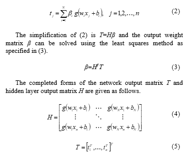
For a given n training set samples (x_j, t_j) where x_j=[x_j1, x_j2,…, x_jn]^T and t_j=[t_j1, t_j2,…, t_jn]^T, an SLFN with N hidden neurons and an activation function g(x) is expressed as [1,21,26]:

where w_i=[w_i1, w_i2,…, w_in]^T, β_i=[β_i1, β_i2,…, β_in]^T, b_i, and o_j are the connecting weight of the i-th hidden neuron to the input neuron, the connecting weights of the i-th hidden neuron to the output neurons, the bias of the i-th hidden node, and the actual network output with respect to input x_j respectively.

The standard SLFN can minimize the deviation between t_j and o_j, so that (1) can be rewritten as follows.

3.2.  Solar Power Plant

The sun emmits electromagnetics radiation with an effective temperature of 5777 K. Radiant energy, the ammount of energy within the radiation, is spread over the time and measured as radiant power also known as irradiance. The radiant power that reach the Earth surface is normaly measured in square meter through a pyranometer. Extraterrestrial irradiance (EXT) is very observable due to the absence of interference when the radiance traveling thru the space. The amount of irradiance reaching the earth’s surface is approximately 1361.1 W/m², which is also known as global horizon irradiance (GHI) expressed in terms of clear-sky irradiance and is one of the most useful variables to calculate when working with solar data. This variable represents the best scenario for a photovoltaic system since it represents the maximum that could be received on the day, resulting in uninterrupted generation [2].

A solar power plant has at least one solar panel to convert energy directly from the sun. An inverter is also required to meet the output needs, and some accessories are involved to protect the process. The energy from a solar power plant depends on solar irradiation, while the constant parameters in calculating output power are the covered area and efficiency of the solar PV modules. Therefore, the output power of a solar power plant is formulated as follows [27].

Where P_PV, A_c, Sir, and h are output power (W) dimension of solar PV modules (m²), number of PV modules, solar irradiance (W/m²) and efficiency of the solar PV modules.

3.3.  Forward Backward Method

The voltage, power, and power loss in a radial distribution network are calculated in this research using the forward backward approach. This approach was created by reference [29] as it is described in their paper. By figuring out three fundamental computations, this method expands on the Distflow method to finish the analysis of power flow in distribution networks. The computations are used to determine the voltage magnitude, active power, and reactive power.

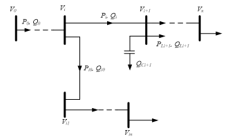
Figure 1: Single line diagram of a general distribution system

Consider the balanced three-phase, radial distribution feeder in Figure 1 with n branches/nodes and nc shunt capacitors. Without a branch from V_k to V_kn on the figure, the power and voltage at each node from V₀ to V_n can be calculated by the following equations [28–30].

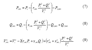
Where P_Li+1 and Q_Li+1 are loads connected at node i+1; P_i+1 and Q_i+1 are the effective real and reactive power flows from node i+1; r_i+1 and x_i+1 are resistance and capacitance of the line leading to bus i+1; P_i and Q_i are real and reactive power flowing from bus i; V_i and V_i+1 are the voltage magnitudes on bus i and bus i+1; and Q_Ci+1 is an additional reactive power of the capacitor on the bus i+1.

The aforementioned equations are referred to as the forward equation, and each procedure is referred to as a forward update. Other calculating techniques and sequences in the Distflow are known as “backward updates” and “backward equations.” The initial values of P₀ and Q₀ in this approximation method are determined by summing the active and reactive power of loads. V₀ is the initial voltage, which is also utilized as the system’s base voltage in the approach method’s calculation procedure [29]. The parameters in the bracket of equations (7) and (8) denote active and reactive power losses. At the end of each branch, the active and reactive power should be equal to zero [28–30].

3.4.  Optimal Power Flow

An important method for improving a system’s performance and lowering operational costs is optimization. A power system subject to dispersing loads amongst power plants is called optimal power flow (OPF). It is possible to decrease the overall fuel cost of all committed plants while still adhering to network limits. The OPF problem was generally expressed as follows [31–33]:

Where f, g and h are the objective functions, the equality constraints represent power flow equations and the system operating constraints, respectively.

The vector x is the dependent variable and consists of the voltage magnitude of load buses, the phase angle of all buses except that of the slack bus, the active power of the slack generator, and generators’ reactive power. The vector of x is also called a state variable, and it is formulated in the following equation:

The vector u is a control variable that includes the active output power of generators at generator buses P_G, the terminal voltage magnitude at generation bus bars V_G, the output of shunt VAR compensators Q_C, and the tap setting of the tap regulating transformers T. Therefore, the vector u can be modeled as follows:

Where S_l is transmission line loading and the subscripts NL, TL, NG, NC, and NT denote the number of load buses, transmission lines, generators, shunt VAR compensators, and regulating transformers, respectively.

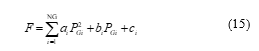
The objective function in an OPF problem is to minimize the generators’ costs in the operations. The cost function represents the relationship between operating costs and output power as expressed in equation (15), where a_i, b_i, and c_i are the coefficients of the fuel cost model.

There are certain equality and inequality restrictions in the problem of optimal power flow. The power flow equations are represented by the equality constraints g, as computed as follows:

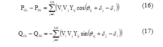
Where P_Gi and Q_Gi are the i-th generator’s active and reactive power; P_Di and Q_Di are the i-th bus’s active and reactive demand. V_i and V_j are the voltage magnitudes at buses i and j; Y_ij models the element of the admittance bus matrix at row i and column j; NB is the number of buses; d_i, d_j, and q_ij are the angels of V_i, V_j, and Y_ij, respectively.

The inequality constraint h limits the physical devices as well as system security. The inequality constraints consist of generator constraints in equations (18) to (20), transformer constraints in equation (21), and shunt capacitor constraints in equation (22). System security constraints, on the other hand, are given in equations (23) and (24).

Where P_Gi^min and P_Gi^max are the minimum and maximum active power of i-th generator and Q_Gi^min and Q_Gi^max denote the minimum and maximum reactive power of i-th generator; S_ij and S_ij^max are line flow and maximum line flow between bus i and j.

3.5.  Model Validation

The developed model needs to be evaluated in order to detect and prevent any potential problems that might appear after running the ELM model. The mistakes will be eliminated through the validation process, making the model sufficiently precise for the simulation to match reality as predicted. The model is verified using the mean absolute error (MAE). It can be expressed as follows [4]:

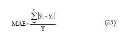
Where ŷ_i, y_i and Y are forecasting data, real data and number of samples, respectivelly.

4. Result and Discussion

4.1.  Datasets

NASA [34] provided the datasets used to train the ELM model, which are located at latitude -0.8457 and longitude 134.0504. The data is based on Modern-Era Retrospective analysis for Research and Applications, Version 2 (MERRA-2) that starts to provide data from 1980. The elevation from MERRA-2 is average for a 0.5 x 0.625 degree latitude/longitude region about 944.25 meters. For the entire year 2021, there are 8016 data items in the dataset for both solar irradiance and ambient temperatures. The solar irradiance data ranges from 0 to 1033.38 Wh/m², which is clear-sky surface shortwave downward irradiance combined with the all-sky insolation clearness index. In same way the ambient temperature ranges from 18.47 to 26.5 ^°C, which is the MERRA-2 temperature at 2 meters.  The model can be used in the research area based on location-specific data. In fact, the model can be used in any other field that has the necessary data for the defined domains and is available to be trained.

4.2.  Training and Validation

The training is carried out using the Windows X-compatible MatLab 2021b program. The PC’s hardware includes a Core i7-2600 CPU running at 3.40 GHz with 4 GB of RAM.

The datasets of 8016 from NASA are used to train the ELM model. The training time of 4.4375 seconds demonstrates the ELM’s superiority, and its precision is sufficient, as indicated by a little modest MAE value. The test data is made up of data for 24 hours, which is the average amount of time for the entire year 2021. Training and testing with 5000 neurons take approximately 4.4375 seconds and 0.0625 seconds, respectively. The validation of the model was done using mean absolute error (MAE), with an error of about 0.6392 for the developed model.

4.3.  Simulations

The simulations are performed to forecast the Manokwari region’s daily solar irradiation and ambient temperatures. Then the results are presented in Figures 2 to 5.

The distribution of solar irradiation data is depicted in Figure 2 as fluctuating between 0 and a maximum of 1022.9 Wh/m². On the other side, hourly fluctuations occur at 14:00, when the difference between the minimum and maximum is rather large, measuring about 142.45 Wh/m². The graph also demonstrates that the forecasted results were located within these gaps [1].

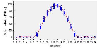
Figure 2: Solar irradiation distribution

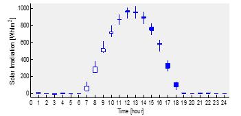
Figure 3: Forecasting of solar irradiation

As shown in Figure 3, a candlestick diagram is used to present the data between the minimum and maximum as well as factual and forecasted data. A thin line in this graph joins the minimum and maximum data points. On the other side, a thick line connects the error rate, which is the discrepancy between the actual and forecasted data. According to the simulation results in Figure 3, the highest error rate occurs at 8:00, around 55.75 Wh/m². The thick line is currently white, implying that the difference is negative in size as a result of the projected result being greater than the actual data  [1].

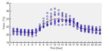
Figure 4: Ambient temperature distribution

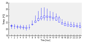
Figure 5: Forecasting of ambient temperature

The ELM model also outputs ambient temperature in accordance with solar irradiation forecasts. The forecasted environmental temperatures are given in Figures 4 and 5 [1]. As seen in Figure 4, the data distribution simultaneously displays a relatively significant variation in the Manokwari region, in contrast to the distribution of data from solar irradiation. This region is close to the equator and directly adjacent to the Pacific Ocean, which indicates a considerable change in environmental circumstances.

The candlestick diagram in Figure 5 depicts data changes between maximum and minimum data for the remainder of the year, with the highest data difference occurring at noon and being 4.02 ^°C. The figure also shows the discrepancy between the actual and anticipated data, with the largest variance of approximately 1.10 ^°C occurring around 16:00  [1].

4.4.  Model Performances

Using the same ELM data for both training and testing, a straightforward feedforward neural network (FFNN) is used to assess the model’s performance. The results of the performance test indicate that more than 1000 neurons cannot be operated on the same machine, while the FFNN requires 203.3281 seconds for training and 0.1250 seconds for testing. The average deviations for both approaches are 0.03 ^°C and 0.28 Wh/m², respectively  [1]. The comparisons revealed that the ELM model has the same accuracy as the FFNN in extremely fast computing.

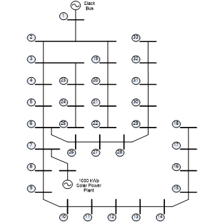
Figure 6: Single line diagram

4.5.  Power Losses Minimization

Surrounding the research location, a distribution line, namely the Rajawali feeder, is operated. The feeder consists of 33 load buses connected to 32 lines, as figured in Figure 6, with data attached in Tables 1 and 2 [29].

Based on Figure 6, it can be seen that the distribution lines are connected in a radial connection. The longest line is from bus 1 to bus 18, where some tabs are taken from bus 6 to connect buses 26 and 33 and a tab is added for the solar power plant penetration. The other branches of the feeder are taken from bus 2 to connect buses 19 and 22 and from bus 3 to connect buses 23 and 25.

Table 1: Bus data

No	Bus Type*	Voltage (pu)	Angle (deg)	Load		Generation
				P (kW)	Q (kVar)	P (kW)	Q (kVar)
1	1	1.00	0.00	0.00	0.00	0.00	0.00
2	2	1.00	0.00	100.00	60.00	0.00	0.00
3	2	1.00	0.00	90.00	40.00	0.00	0.00
4	2	1.00	0.00	120.00	80.00	0.00	0.00
5	2	1.00	0.00	60.00	30.00	0.00	0.00
6	2	1.00	0.00	60.00	20.00	0.00	0.00
7	3	1.00	0.00	200.00	100.00	1000.00	0.00
8	2	1.00	0.00	200.00	100.00	0.00	0.00
9	2	1.00	0.00	60.00	20.00	0.00	0.00
10	2	1.00	0.00	60.00	20.00	0.00	0.00
11	2	1.00	0.00	45.00	30.00	0.00	0.00
12	2	1.00	0.00	60.00	35.00	0.00	0.00
13	2	1.00	0.00	60.00	35.00	0.00	0.00
14	2	1.00	0.00	120.00	80.00	0.00	0.00
15	2	1.00	0.00	60.00	10.00	0.00	0.00
16	2	1.00	0.00	60.00	20.00	0.00	0.00
17	2	1.00	0.00	60.00	20.00	0.00	0.00
18	2	1.00	0.00	90.00	40.00	0.00	0.00
19	2	1.00	0.00	90.00	40.00	0.00	0.00
20	2	1.00	0.00	90.00	40.00	0.00	0.00
21	2	1.00	0.00	90.00	40.00	0.00	0.00
22	2	1.00	0.00	90.00	40.00	0.00	0.00
23	2	1.00	0.00	90.00	50.00	0.00	0.00
24	2	1.00	0.00	420.00	200.00	0.00	0.00
25	2	1.00	0.00	420.00	200.00	0.00	0.00
26	2	1.00	0.00	60.00	25.00	0.00	0.00
27	2	1.00	0.00	60.00	25.00	0.00	0.00
28	2	1.00	0.00	60.00	20.00	0.00	0.00
29	2	1.00	0.00	120.00	70.00	0.00	0.00
30	2	1.00	0.00	200.00	600.00	0.00	0.00
31	2	1.00	0.00	150.00	70.00	0.00	0.00
32	2	1.00	0.00	210.00	100.00	0.00	0.00
33	2	1.00	0.00	60.00	40.00	0.00	0.00
*Type of bus: 1:slack; 2:load; 3:generator

Table 2: Line data

No		Line (From – To)			Impedance (Ohm)						No		Line (From – To)		Impedance (Ohm)
					R			jX							R	jX
1		1 – 2			0.0922			0.0470			17		14 – 15		0.5910	0.5260
2		2 – 3			0.4930			0.2511			18		15 – 16		0.7463	0.5450
3		2 – 19			0.1640			0.1565			19		16 – 17		1.2890	1.7210
4		3 – 4			0.3660			0.1864			20		17 – 18		0.7320	0.5740
5		3 – 23			0.4512			0.3083			21		19 – 20		1.5042	1.3554
6		4 – 5			0.3811			0.1941			22		20 – 21		0.4095	0.4784
7		5 – 6			0.8190			0.7070			23		21 – 22		0.7089	0.9373
8		6 – 7			0.1872			0.6188			24		23 – 24		0.8980	0.7091
9		6 – 26			0.2030			0.1034			25		24 – 25		0.8960	0.7011
10		7 – 8			0.7114			0.2351			26		26 – 27		0.2842	0.1447
11		8 – 9			1.0300			0.7400			27		27 – 28		1.0590	0.9337
12		9 – 10			1.0440			0.7400			28		28 – 29		0.8042	0.7006
13		10 – 11			0.1966			0.0650			29		29 – 30		0.5075	0.2585
14		11 – 12			0.3744			0.1238			30		30 – 31		0.9744	0.9630
15		12 – 13			1.4680			1.1550			31		31 – 32		0.3105	0.3619
16		13 – 14			0.5416			0.7129			32		32 – 33		0.3410	0.5302

A solar power plant has been prepared to be installed on the Rajawali feeder, which is planned to be integrated into the grid through the feeder. The power plant has an output power of 1000 kW, and the plant consists of 3498 PV panels with an output power of 260 Wp. The PV panel data is provided as follows.

Optimum operating voltage (Vmp)	: 30.60 V
Optimum operating current (Imp)	: 8.50 A
Open–circuit voltage (Voc)	:37.70 V
Short–circuit current (Isc)	: 9.15 A
Maximum power (Pmax)	: 260 W
Efficiency	:16 %
Operating module temperature	: -40 to 85 °C
Maximum system voltage	:1000 VDC
Maximum series fuse rating	:15 A
Power tolerance	: 0–3%
Solar cell type	: Monocrystalline
Number of cells	: 60
Dimensions (mm)	: 1636x992x45

The solar power plant will be used as a model to investigate the use of ELM forecasting results to investigate the penetration effect of the solar power plant in increasing the voltage profile and thus improving power losses. The results will be compared with the existing operating conditions, which probably have high power losses in operation.

The simulation is carried out using forecasting data from both NN and ELM methods. The forecasting results will then be converted into electrical energy, which will be integrated into the grid according to the specifications of the solar panels used and calculated using equation (6). The results of hourly load forecasting will also be influenced by the pattern of changes in load on each bus, which varies according to peak load times. The simulation results show an improvement in the voltage profile and power loss, as shown in Tables 3 and 4, and also illustrated in Figure 7.

Table 3: Average voltage magnitude (p.u.) and load profile (kW)

Bus	Existing	NN	ELM	Load	Bus	Existing	NN	ELM	Load
1	1.000	1.000	1.000	135.06	18	0.928	0.941	0.941	59.64
2	0.997	0.998	0.998	85.47	19	0.995	0.996	0.996	74.16
3	0.986	0.987	0.987	120.79	20	0.992	0.991	0.991	84.24
4	0.983	0.985	0.985	66.00	21	0.990	0.990	0.990	93.02
5	0.976	0.981	0.981	96.91	22	0.989	0.989	0.989	80.38
6	0.968	0.978	0.978	80.29	23	0.985	0.984	0.984	73.44
7	0.963	0.984	0.984	99.46	24	0.983	0.978	0.978	133.77
8	0.955	0.976	0.976	113.71	25	0.983	0.975	0.975	63.01
9	0.954	0.970	0.970	73.32	26	0.962	0.974	0.974	88.08
10	0.953	0.965	0.965	94.15	27	0.961	0.971	0.971	67.16
11	0.948	0.962	0.962	73.55	28	0.956	0.960	0.960	65.13
12	0.941	0.958	0.958	69.21	29	0.953	0.952	0.952	62.47
13	0.936	0.951	0.951	85.46	30	0.951	0.948	0.948	65.37
14	0.935	0.949	0.949	69.00	31	0.949	0.944	0.944	77.83
15	0.933	0.947	0.947	82.24	32	0.948	0.943	0.943	78.92
16	0.929	0.944	0.944	140.82	33	0.948	0.942	0.942	99.92
17	0.928	0.942	0.942	98.08	Avg	0.962	0.968	0.968	86.37

The outer buses on the feeder are those of 18, 22, 25, and 33, which have the lowest average voltage on the lines. After the penetration of the solar power plant, the average voltages are increasing on the buses, except for bus number 22, which is highly influenced by the slack bus voltage, as shown in Table 3. Overall, the average voltage of the feeder is increased by the solar power plant from 0.962 to 0.968 for both NN and ELM forecasting. The voltage profile improvement also occurs in many cases of power plant injection into a grid, which acts as a distributed generator, as reported in references [9–11,14,17].

Table 4: Power Loss Minimization (kW)

Time	Existing	NN	ELM	Time	Existing	NN	ELM
1	1.4050	1.4050	1.4050	14	1.6290	1.0760	0.4550
2	1.4270	1.4270	1.4270	15	1.6020	1.0760	0.4660
3	1.4110	1.4110	1.4110	16	1.5960	1.0760	0.4560
4	1.4810	1.4810	1.4810	17	1.5510	1.0760	0.4560
5	1.4840	1.4840	1.4840	18	1.5460	1.0760	0.4480
6	1.4960	1.0760	0.4270	19	1.5640	1.5640	1.5640
7	1.5020	1.0760	0.4320	20	1.5060	1.5060	1.5060
8	1.5210	1.0760	0.4320	21	1.4780	1.4780	1.4780
9	1.5060	1.0760	0.4380	22	1.4020	1.4020	1.4020
10	1.5270	1.0760	0.4350	23	1.4050	1.4050	1.4050
11	1.5960	1.0760	0.4420	24	1.4020	1.4020	1.4020
12	1.5980	1.0750	0.4580	S	36.2280	29.9520	21.7640
13	1.5930	1.0760	0.4540	%	100.0000	17.3236	39.9249

The data in Table 4 shows that at night, the power loss forecast for the line will be the same as the existing condition. Therefore, the power loss simulation is carried out using the forward backward sweep (FBS) method. Furthermore, when the sun starts to shine, the power loss is analyzed by the Optimal Power Flow (OPF) method. This is a fact of the system because it is a pure radial distribution system without solar power penetration. Then the power loss problem needs to be solved with the FBS method because it will cause simulation calculation errors with the OPF method that is used for a complex power system. In a different way, during the day, there is energy penetration on the system’s bus 7, transforming the system into a multi-machine system connected to a radial distribution system, where power loss problems should be counted using the OPF method.

When the solar power starts to penetrate at 6 a.m., the ELM simulation shows a decrease in power loss until it reaches a maximum at around 12 p.m., and after noon, the power loss slowly increases as the solar radiation reaching the PV panel is reduced. The ELM method is smaller than the NN method because the ELM prediction gives more accurate results compared to the NN forecast, which yields a high percentage of power loss minimization. Data on the table shows that average power loss without solar power penetration is about 1.5095 kW/hour, which is reduced in average by the penetration of about 1.2480 kW/hour and 0.9068 kW/hour of NN and ELM forecasting, respectively.

On the other hand, the simulation results show that the power loss simulated through NN forecasting tends to be constant throughout the solar power plant’s operation. This resulted in less solar power penetration, and its contribution to the power loss is also less, as indicated by the small percentage of power loss, which is only 17.3236 % compared to the ELM forecasting percentage that reached 39.9249 %.

The standard deviations of power losses have decreased from 6.9441 in the existing condition to 5.7440 and 4.2015 for both NN and ELM, respectively. This indicates that the performance of the system has improved with the penetration of solar power plants. However, the smallest standard deviation values indicate that power loss minimization represents a more accurate result of the ELM algorithm.

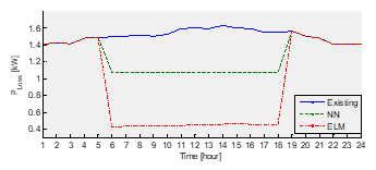
Figure 7: Power losses improvement

Figure 7 depicts the difference in power loss for the following day of the normal calculation versus the improved results due to the penetration of the 1000 kWp solar power plant on bus 7. The figure shows that there is a high power loss improvement predicted with ELM compared to the NN prediction, which tends to be stable throughout the operating time of the solar power plant. The prediction results show the accumulated power loss through NN predictions of 29.9520 kW and ELM predictions of 21.7640 kW, which is slightly lower than the normal calculation of about 36.2280 kW. This prediction result is not high for predictions in the day ahead, but it will change significantly for long-term forecasting.

Overall, the proposed method is done in the sequence of forecasting solar irradiation a day ahead in [1], injecting the solar irradiation into a power grid, calculating power flow in the grid, and investigating the power losses by comparing the results with another method. It is found that by applying the proposed method in a microgrid system, the average voltage is raised to 0.968 p.u. and further power losses in day-ahead operation can be minimized to 0.79% of the total load of 2763.84 kW. The proposed method is also valid in terms of accuracy as measured by standard deviation.

5. Conclusions

In this study, an ELM model has been developed to forecast solar data for the following day as well as data on the ambient temperature. The ELM model includes 5000 neurons in the hidden layer and was trained using annual datasets of about 8016 items. The forecasting process takes 0.0625 seconds, while training takes 4.4375 seconds of CPU time. The model has been verified using the MAE approach and has a relatively low error rate of 0.6392, making it considered accurate enough to be used to forecast solar irradiation and the surrounding air temperature at the sampling sites. The ELM model’s performances have also been compared with those of a straightforward feed-forward neural network (FFNN), which has the same accuracy but requires less time to train and evaluate.

Power loss minimization for the day-ahead operation of a 1000 kWp solar panel based on the ELM data forecasting can reach 21.7640 kW, or about 39.9249 percent, compared to the existing operation without solar penetration of about 36.2280 kW. The power loss is reduced by the penetration of the solar power plant from 1.5095 kW/hour to 0.9068 kW/hour.

Acknowledgment

The first author would like to thank his colleagues from Electrical Engineering Department, Engineering Faculty of Papua University, Manokwari, who provided insight and expertise that greatly assisted this research.

1. A.B. Rehiara, S. Setiawidayat, “Day Ahead Solar Irradiation Forecasting Based on Extreme Learning Machine,” in 2022 IEEE International Conference on Cybernetics and Computational Intelligence (CyberneticsCom), 63–66, 2022, doi:10.1109/CyberneticsCom55287.2022.9865532.
2. J.M. Bright, Introduction To Synthetic Solar Irradiance, 1-1-1–32, doi:10.1063/9780735421820_001.
3. B. Brahma, R. Wadhvani, “Solar Irradiance Forecasting Based on Deep Learning Methodologies and Multi-Site Data,” Symmetry, 12(11), 2020, doi:10.3390/sym12111830.
4. M. Abdillah, W.A. Pramudito, T.A. Nugroho, D.N. Fitria, “Solar irradiance forecasting using kernel extreme learning machine: case study at Lamongan and Muara Karang regions, Indonesia,” 17, 2022.
5. V.V.V.S.N. Murty, A. Kumar, “Optimal Energy Management and Techno-economic Analysis in Microgrid with Hybrid Renewable Energy Sources,” Journal of Modern Power Systems and Clean Energy, 8(5), 929–940, 2020, doi:10.35833/MPCE.2020.000273.
6. D. Sampath Kumar, O. Gandhi, C.D. Rodríguez-Gallegos, D. Srinivasan, “Review of power system impacts at high PV penetration Part II: Potential solutions and the way forward,” Special Issue on Grid Integration, 210, 202–221, 2020, doi:10.1016/j.solener.2020.08.047.
7. S. Monshizadeh, “Comparison of Intelligent Algorithms with FACTS Devices for Minimization of Total Power Losses,” Advances in Intelligent Systems and Computing, 926(Query date: 2022-12-02 17:21:04), 120–131, 2020, doi:10.1007/978-3-030-15032-7_10.
8. S.P. Dash, “Optimal location and parametric settings of FACTS devices based on JAYA blended moth flame optimization for transmission loss minimization in power systems,” Microsystem Technologies, 26(5), 1543–1552, 2020, doi:10.1007/s00542-019-04692-w.
9. A. Alam, “Optimal placement of DG in distribution system for power loss minimization and voltage profile improvement,” 2018 International Conference on Computing, Power and Communication Technologies, GUCON 2018, (Query date: 2022-12-02 17:21:04), 837–842, 2019, doi:10.1109/GUCON.2018.8674930.
10. S. Essallah, “Optimal Multi-Type DG Integration and Distribution System Reconfiguration for Active Power Loss Minimization using CPSO Algorithm,” 2019 International Conference on Control, Automation and Diagnosis, ICCAD 2019 – Proceedings, (Query date: 2022-12-02 17:21:04), 2019, doi:10.1109/ICCAD46983.2019.9037947.
11. G.A.S. Gandhi, “Optimal allocation of DG for minimization of power loss and total investment cost using an analytical approach,” 2020 21st National Power Systems Conference, NPSC 2020, (Query date: 2022-12-02 17:21:04), 2020, doi:10.1109/NPSC49263.2020.9331891.
12. S. Ansari, J. Zhang, R.E. Singh, “A review of stabilization methods for DCMG with CPL, the role of bandwidth limits and droop control,” Protection and Control of Modern Power Systems, 7(1), 2, 2022, doi:10.1186/s41601-021-00222-x.
13. N. Pragallapati, S.J. Ranade, O. Lavrova, “Cyber Physical Implementation of Improved Distributed Secondary Control of DC Microgrid,” 2021 1st International Conference on Power Electronics and Energy (ICPEE), doi:10.1109/icpee50452.2021.9358705.
14. M. Kang, “Optimal placement and sizing of DG and shunt capacitor for power loss minimization in an islanded distribution system,” Lecture Notes of the Institute for Computer Sciences, Social-Informatics and Telecommunications Engineering, LNICST, 245(Query date: 2022-12-02 17:21:04), 43–52, 2018, doi:10.1007/978-3-319-94965-9_5.
15. M.B. Essa, “Distribution power loss minimization via optimal sizing and placement of shunt capacitor and distributed generator with network reconfiguration,” Telkomnika (Telecommunication Computing Electronics and Control), 19(3), 1039–1049, 2021, doi:10.12928/TELKOMNIKA.v19i3.15223.
16. D. Bhowmik, “Optimal placement of capacitor banks for power loss minimization in transmission systems using fuzzy logic,” Journal of Engineering Science and Technology, 13(10), 3190–3203, 2018.
17. S. Nawaz, “A new technique to solve DG allocation problem for distribution power loss minimization,” ICIC Express Letters, Part B: Applications, 9(7), 701–706, 2018, doi:10.24507/icicelb.09.07.701.
18. N.T. Rao, “Comparative study of Pareto optimal multi objective cuckoo search algorithm and multi objective particle swarm optimization for power loss minimization incorporating UPFC,” Journal of Ambient Intelligence and Humanized Computing, 12(1), 1069–1080, 2021, doi:10.1007/s12652-020-02142-4.
19. M. Sankaramoorthy, “A hybrid MACO and BFOA algorithm for power loss minimization and total cost reduction in distribution systems,” Turkish Journal of Electrical Engineering and Computer Sciences, 25(1), 337–351, 2017, doi:10.3906/elk-1410-191.
20. N. Vazquez, “A Fully Decentralized Adaptive Droop Optimization Strategy for Power Loss Minimization in Microgrids with PV-BESS,” IEEE Transactions on Energy Conversion, 34(1), 385–395, 2019, doi:10.1109/TEC.2018.2878246.
21. R. Adelhard Beni, C. He, S. Yutaka, Y. Naoto, Z. Yoshifumi, “An Adaptive Internal Model for Load Frequency Control Using Extreme Learning Machine,” TELKOMNIKA, 16(6), 2879–2887, 2018, doi:http://dx.doi.org/10.12928/telkomnika.v16i6.11553.
22. Y. Lu, W. Yu, J. Wang, D. Jiang, R. Li, “Design of PID Controller Based on ELM and Its Implementation for Buck Converters,” International Journal of Control, Automation and Systems, 19(7), 2479–2490, 2021, doi:10.1007/s12555-019-0989-1.
23. P. Winangun, I.M. Widyantara, R. Hartati, “Extreme Learning Machine Based Diagnostic Approach with Linear Kernel for Classifying Lung Disorders,” Majalah Ilmiah Teknologi Elektro, 19(1), 83–88, 2020, doi:10.24843/MITE.2020.v19i01.P12.
24. C. Jia, H. Zhang, “ELM Neural Network-based Fault Diagnosis Method for Mechanical Equipment,” in 2019 Chinese Automation Congress (CAC), 5257–5261, 2019, doi:10.1109/CAC48633.2019.8996333.
25. M.N. dan I.C. dan I. Indriati, “Stock Price Earning Ratio Prediction Using the Kernel Extreme Learning Machine Algorithm (Case Study: PT TELKOM),” Jurnal Pengembangan Teknologi Informasi Dan Ilmu Komputer, 4(10), 3455–3462, 2020.
26. G. Huang, S. Song, J.N.D. Gupta, C. Wu, “Semi-Supervised and Unsupervised Extreme Learning Machines,” IEEE Transactions on Cybernetics, 44(12), 2405–2417, 2014, doi:10.1109/TCYB.2014.2307349.
27. F. Odoi-Yorke, A. Woenagnon, “Techno-economic assessment of solar PV/fuel cell hybrid power system for telecom base stations in Ghana,” Cogent Engineering, 8(1), 1911285, 2021, doi:10.1080/23311916.2021.1911285.
28. S.F. Mekhamer, S.A. Soliman, M.A. Mostafa, M.E. El-Hawary, “Load flow solution of radial distribution feeders: a new approach,” in 2001 IEEE Porto Power Tech Proceedings (Cat. No.01EX502), 3, 5, 2001, doi:10.1109/PTC.2001.964918.
29. B.R. Wihyawari, “Radial Power Flow Analysis of Rajawali Feeder in Manokwari Power Grid,” in ICTVT 2021, State University of Yogyakarta, 2021.
30. J.A.M. Rupa, S. Ganesh, “Power Flow Analysis for Radial Distribution System Using Backward/Forward Sweep Method,” International Journal of Electrical and Computer Engineering, 8(10), 1628–1632, 2014.
31. A.B. Rehiara, “Optimal Power Flow of the Manokwari Power Grid Regarding Penetration of 20 MW Combined Cycle Power Plant,” in 2019 International Conference on Advanced Mechatronics, Intelligent Manufacture and Industrial Automation (ICAMIMIA), 53–57, 2019, doi:10.1109/ICAMIMIA47173.2019.9223393.
32. L.T. Al-Bahran, A.Q. Abdulrasool, “Multi objective functions of constraint optimal power flow based on modified ant colony system optimization technique,” IOP Conference Series: Materials Science and Engineering, 1105(1), 012015, 2021, doi:10.1088/1757-899X/1105/1/012015.
33. H. Bouchekara, “Solution of the optimal power flow problem considering security constraints using an improved chaotic electromagnetic field optimization algorithm,” Neural Computing and Applications, 32(7), 2683–2703, 2020, doi:10.1007/s00521-019-04298-3.
34. NASA, NASA/POWER CERES/MERRA2 Native Resolution Hourly Data, 2021.

(Click Here)