1. Introduction

The Activity and Event Network (AEN) is a new graph that models a computer network by capturing various network security events that occur in the network perimeter. The AEN has the purpose of providing a base for the detection of both novel and known attack patterns, including long-term and stealth attack methods, which have been on the rise but have proven difficult to detect.

This paper is an extension of work originally presented in the 3rd Workshop on Secure IoT, Edge and Cloud systems (SIoTEC) of the 22nd IEEE International Symposium on Cluster, Cloud and Internet Computing (CCGrid 2022) [1]. In the present paper, we present an unsupervised ensemble intrusion detection mechanism composed of two detection schemes, one signature-based and one anomaly-based, with the goal of leveraging the strengths of both types of detection methods and mitigating their weaknesses.

Signature-based detection, also known as rule-based detection, works by searching data for specific characteristics of previously seen attacks. This makes it good at detecting known attack patterns, but at the same time renders it ineffective when confronted with new and unseen attacks. In contrast, anomaly detection methods rely on the assumption that events deviating from normal usage patterns or behaviours are potentially malicious. This method has the potential to detect novel attack patterns but may generate a large number of false positives due to the fact that atypical events are not necessarily malicious [2, 3].

To validate the scheme, we provide a collection of attack fingerprints covering a small subset of known scanning, denial of service (DoS) and password guessing attacks.

The fingerprints are described using Property Graph Query Language (PGQL) because it provides a standardized language for describing graphical patterns, which we believe makes comprehension easier than describing the fingerprints algorithmically. We also provide a subgraph matching algorithm specifically for finding subgraphs that are isomorphic to the fingerprints.

The anomaly-based scheme, in turn, involves calculating anomaly scores based on the bits of meta-rarity metric introduced by [4] for a set of 15 statistical features and underlying distributions extracted from the AEN graph.

To evaluate the proposed intrusion detection mechanism, we conducted experiments with two datasets: the Information Security and Object Technology (ISOT) Cloud Intrusion Detection (ISOT-CID) Phase 1 dataset [5] and the 2017 Canadian Institute for Cybersecurity (CIC) Intrusion Detection Evaluation Dataset (CIC-IDS2017) [6]. First, each of the two schemes were separately evaluated, and then an ensemble classification was created that fuses the two results. The obtained results were promising for both the individual detection schemes and for the combined method.

The remainder of this paper is structured as follows. In section 2, we review the literature on graph-based intrusion detection, anomaly detection and subgraph matching. In section 3 we give a brief overview of the AEN graph. In section 4, we present the fingerprint model and explain how the fingerprints are described and searched for in the graph. In section 5, we provide detail about the anomaly detection model, including a description of the anomaly score calculation and the proposed features model. In section 6, we present the experimental evaluation of the proposed scheme and discuss the obtained performance results. Finally, in section 7, we make concluding remarks.

2. Literature Review

2.1. Graph-based Intrusion Detection

Many different graphical models have been proposed for intrusion detection or forensic analysis. One traditional focus is on nonprobabilistic models, such as attack graphs. These include state attack graphs [7]–[9], logical attack graphs [10] and multiple prerequisite graphs [11], each of which aims to either elucidate different aspects of the system or network’s security issues or, at a minimum, fix the limitations of the previous models. In general, there are many open challenges when working with attack graphs [12].

Current approaches are plagued by the exponential growth of the graph according to its vulnerabilities and network size, making generation intractable, even for a few dozen hosts. They are limited in scope, and while they provide static information about the attack paths and the probability of a vulnerability exploitation, they do not provide any information about other effective parameters, such as current intrusion alerts, active responses or network dependencies. Furthermore, current attack graphs do not capture the dynamic and evolving nature of the long-term threat landscape. In practice, each change to the network requires a complete recreation of the graph and a restart of the analysis, which means they can only be applied for offline detection.

Another important area of research is in probability or beliefbased models used for signature-based intrusion detection such as those employing Bayesian networks (BNs) [13]–[15] and Markov random fields (MRFs) [16, 17]. These models provide good results for the modelled attacks but have some important limitations. The first stems from the fact that the entity being modelled is not the network itself. Instead, the graph is constructed based on predefined features, which limits the extensibility of the models. This is because each new attack type requires the definition of more predefined features that must be incorporated into the graph as new elements. Moreover, these methods require a training phase used to define the graph’s probabilities, making them fully supervised methods. Finally, like attack graphs, they need to be reconstructed whenever the graph changes, which can be time consuming, and in practice make them unable to perform online detection.

Moving to anomaly detection applied for intrusion detection, numerous models have been proposed that have used a diverse range of techniques, such as decision trees [18] and neural networks [19]–[21]. These models obtain good performance but suffer from the previously mentioned issues, including necessitating a training phase, requiring multiple rounds of training in some cases, and not supporting online detection. Moreover, despite being anomalybased, some models have a limited capability to identify novel attacks due to their structure based on predefined features.

In our work we overcame these problems by modelling the network itself. This allows for greater extensibility in describing new attacks because, rather than attack features being predefined, they may be extracted from the graph. Moreover, the AEN graph is fully dynamic and in constant change. Each new subgraph matching operation can be performed against the graph online without the need to recreate it after every change. Finally, the proposed schemes are all unsupervised, which eliminates the need for a training phase.

2.2. Isomorphic Subgraph Matching

Isomorphic subgraph matching is used to search graphs for subgraphs that match a particular pattern. It has been employed extensively in diverse areas, including computer vision, biology, electronics and social networks. However, to the best of our knowledge, our work is the first to employ isomorphic subgraph matching for signature-based intrusion detection.

The general form of this problem is known to be NP-complete [22]; however, its complexity has been proven to be polynomial for specific types of graphs, such as planar graphs [23].

Different algorithms have been proposed for this problem. For example, Ullmann’s algorithm [24] uses a depth-first search algorithm to enumerate all mappings of the pattern. Over the years, many improvements have been proposed for that algorithm, such as the VF2 algorithm [25], in attempts to more effectively prune search paths. More modern algorithms, such as the Turboiso [26] and the DAF [27], employ pre-built auxiliary indexes to accelerate searches and facilitate search-space pruning. These algorithms can perform several orders of magnitude faster than index-less algorithms like Ullmann’s but require more memory to store the index and also some pre-processing time to build the indexes.

In our work, we leveraged these ideas to design a custom-made matching algorithm specifically to match fingerprints, given the specific characteristics of the AEN and the proposed fingerprints.

3. AEN Graph Overview

The AEN graph was designed to model the variety, complexity and dynamicity of network activity, along with the uncertainty of its data, something that is intrinsic to the collection process, through a time-varying uncertain multigraph. The graph is composed of different types of nodes and edges, with the nodes describing different types of network elements, such as hosts, domains and accounts, and the edges describing their relationships, such as sessions (sets of traffic between two hosts of the same protocol, ports, etc.) and authentication attempts (an account trying to authentication on a host). Furthermore, each element type has different sets of properties, including domain name, account identifier, session protocol and start and stop time. To build such a graph, data from heterogeneous sources (e.g. network traffic, flow data) and system and application logs (e.g. syslog, auditd) are used.

The graph is built online, with elements added or modified as soon as they are observed in the data and old elements removed once they are considered stale. Consequently, the graph serves as a stateful model of the network, and as such, can be used as a basis for many different types of analyses and inferences. Interested readers are referred to [28] for more details on the AEN graph model’s elements and construction.

4. Attack Fingerprints in the AEN Graph Model

4.1. AEN Fingerprints Framework

4.1.1       Attack Fingerprint Visualization

As a visual example of how attack fingerprints can be mined from the AEN graph, Figure 1 shows how certain network activity can create evident patterns in the graph. Specifically, the figure shows a visualization of a subset of a graph generated from an example dataset containing a distributed password guessing attack. The hosts are represented by blue nodes at the center, accounts that were used in authentication attempts are represented by orange nodes and the attempts themselves (edges) are either blue when successful or orange when unsuccessful.

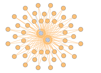
Figure 1: Visualization of an AEN graph containing a password guessing attack.

The figure shows a “cloud” of failed authentication attempts against the two central hosts using the same set of accounts. Furthermore, the majority of the edges are orange, indicating failed attempts, but there is a single blue (successful) edge. This pattern makes evident a successful combined credential stuffing and spraying attack where, after several failed attempts, one login was successful.

Likewise, other types of attacks insert their own distinct attack patterns in the graph. It follows that those patterns serve as fingerprints of these attacks and can, therefore, be mined using subgraph isomorphism matching algorithms to identify instances of an attack.

The statefulness of the AEN plays an important role here because it permits the formation of long term patterns. That is in contrast with traditional intrusion detection systems (IDSs) which can only identify short-term patterns. In the given example, the attack could have been carried out over several weeks, which would have created a challenge for traditional detection mechanisms. In contrast, because the AEN maintains the relationships over a longer term, those patterns can emerge and be identified.

4.1.2       Problem Definition

Given a graph G = (N_G, E_G) where N_G is the set of nodes and E_G : N_G × N_G is the set of edges, the graph F = (N_F, E_F) is isomorphic to a subgraphG′ ofG if all nodes and edges of F can be mapped to nodes and edges of G. More formally, F G if there is a bijective function f : N_F →7 N_G such that ∀u ∈ N_F, f(u) ∈ N_G and ∀(u_i,u_j) ∈ E_F, (f(u_i), f(u_j)) ∈ E_G.

The definition above can easily be extended to apply to more complex graphs that contain labels and properties, such as the AEN, by applying f to those labels and properties as well.

Finally, the problem of matching a fingerprint is defined as the following: Given an AEN graph G and a fingerprint F, find all distinct subgraphs of G that are isomorphic to F.

4.1.3       Describing Attack Fingerprints

In this study, the attack fingerprints are described using the PGQL query language [29] because it provides a standardized language for describing queries, or patterns, that we wish to search for in a property graph. We believe this makes comprehension easier than when the fingerprints are described algorithmically. This is because PGQL’s syntax follows SQL where possible, except that instead of querying tables, it aims to find matches in the nodes and edges of a graph. Doing so requires specific symbols and constructs for that purpose, but is still easily understandable by those who already know SQL.

Other graph query languages, such as Cypher [30], are also descriptive for this purpose but are less like SQL and have a distinct set of supported features. Still, in most cases, PGQL queries can easily be adapted to other graph query languages.

A simple example of PGQL query is as follows:

Algorithm 1: PGQL query example

SELECT s, d

MATCH (s:HOST)-[e:SESSION]->(d:HOST)

WHERE e.duration > 30

The SELECT clause specifies what values are to be returned, while the MATCH clause specifies the pattern to match. The parentheses are used to describe nodes, while the square brackets describe edges, with the arrow specifying the direction, if any. Inside the brackets, the colon separates the variable name to the left and the optional label, or type, to the right. The above example matches any pattern in the graph that involves two nodes, s and d, of type HOST connected by a directed edge, e, of type SESSION, from s to d, whose duration is greater than 30, and then returns the two nodes for each match.

In general, PGQL allows for a rich description of graph patterns; however, it has limitations which make it impossible to fully express certain attack patterns and, in particular, the information we wish to retrieve from it. For our specific use case, PGQL has the following key limitations:

1. Subquery is not supported in the FROM clause.
2. There is limited array aggregation support: In some cases, it is desirable to group matches by destination (the victim) and get an array of sources. However, the current PGQL specification supports only array aggregation of primitive types in paths (using the ARRAYAGG function). Therefore, only properties like IDs can be aggregated in this way. Note that there are some cases where only the LISTAGG function is supported. In those cases, we use the ARRAYAGG function to substitute for LISTAGG as if the former had similar support as the latter for simpler pattern description.

To overcome these limitations, the fingerprints contain a postprocessing phase during which the query results are processed to reach a final match result.

4.1.4       Attack Fingerprint Matching

Finding matches to fingerprints in the AEN graph requires the application of an isomorphic matching algorithm. How this is accomplished depends on the graph engine used to store the AEN graph.

In engines that natively support PGQL, such as PGX and Oracle’s RDBMS with the OPG extension, the fingerprints can be used directly to query the database, with only the post-processing phase requiring further implementation. In this case, the matching algorithm is implemented by the graph engine itself.

Similarly, in engines that support other graph query languages, such as neo4j, the fingerprints need first to be converted to the supported query language, but after that, only the post-processing phase requires implementation.

In contrast, when using any graph engine that does not support a graph query language, the whole fingerprint matching algorithm must be implemented. There are several general isomorphic matching algorithms, including Ullmann’s algorithm [24] and its derivations (e.g. VF2 [25]), the Turboiso [26] algorithm and the DAF [27] algorithm. However, the specific characteristics of the AEN graph and the proposed fingerprints means that a simpler searching algorithm can be employed.

Specifically, the small diameter of the fingerprints means that recursion or any type of partial matching is unnecessary, while the types and properties of the nodes and edges allow for large swathes of the search space to be quickly pruned. In practice, the custom graph engine implemented for the AEN speeds up searching at the cost of extra memory by maintaining separate sets of nodes per type, as well as separate sets of edges per type and per source and destination pair. This can be considered analogous to the indexes employed by the general algorithms mentioned previously, such as the Turboiso and the DAF.

Consequently, finding pairs of nodes per type and edges between them is a constant-time operation. Conversely, iterating the set of edges or groups is done linearly because no index per property is maintained. However, this operation can be trivially parallelized.

Aggregating values, such as summing up properties of elements in groups, must also be done linearly.

A generic fingerprint matching algorithm equivalent is presented in Algorithm 2. The algorithm starts by pairing nodes of the desired types (note that each pair is directed). Then, for each pair, it finds all edges between the source and the destination nodes. For each of those edges, the matches function is used to test whether the edge matches all of the WHERE clauses of the fingerprint and then accumulates the matching edges.

Afterwards, edges are grouped into sets according to the GROUP

BY expression specified in the fingerprint. Subsequently, each set

(group) is tested for matches to all of the HAVING clauses of the fingerprint. If true, the results are extracted from the elements in the set based on the SELECT expression. These results map to what is returned by the PGQL queries.

Algorithm 2: Generic fingerprint matching algorithm

pairs ← pairNodes(nodes, srcType, destType) matched ← {}

foreach pair in pairs do

s, d ← pair

edges ← getEdges(s, d, edgeType)

foreach e in edges do

if matches(e, whereClauses) then matched ← matched ∪ {e} groups ← group(matched, groupingExpr) preResults ← {}

foreach g in groups do

if matches(g, havingClauses) then gr ← extractPreResult(g, selectExpr) preResults ← preResults ∪ {gr} return preResults

As mentioned previously, many fingerprints also require a postprocessing phase, for which Algorithm 3 is the generic algorithm used. It returns a set of matches of the fingerprint as described in the respective section of each fingerprint.

Algorithm 3: Generic fingerprint post-processing phase algorithm

postProcGroups ← group(preResults,

postProcGroupingExpr) results ← {}

foreach ppg in postProcGroups do if matches(ppg, postProcClauses) then

r ← extractFinalResult(ppg,

postProcSelectExpr)

results ← results ∪ {r} return results

Finally, as explained in the following sections, some fingerprints employ the sliding window algorithm to define time windows. In those cases, Algorithms 2 and 3 are applied for each time window separately, although it would be straightforward to apply the postprocessing phase to the combined results of all time windows and group them accordingly. Because the consecutive time windows share some elements, it is possible that the same results will appear on different windows. Therefore, an optional final step when the sliding window is used is the deduplication of results in different time windows, which can be applied to the results returned by Algorithm 3.

Also, to speed up searching in those cases, the sets of edges between nodes are sorted by the desired sliding property so that the start and end indexes of each window can be quickly identified through the application of a binary search. Moreover, the algorithm maintains a cursor to the initial position of the previous window so that older elements do not need to be searched.

4.2. Scanning Attacks

Scanning attacks consist of probing machines for openings that can be further explored for vulnerabilities and then exploited. They are part of the initial information gathering phase of an attack.

These attacks can target a variety of protocols and applications but are most commonly employed for scanning TCP and UDP ports [31]. They can be deployed by a single source or be distributed among several attackers. In addition, there are many different techniques used for scanning, with each focusing on different layers and using different methods to avoid detection [32, 31].

Scanning attacks can be classified based on several different properties. With regard to their footprints, they can be classified into three major types [32]:

• Vertical scan, which scans multiple ports on a single host
• Horizontal scan, which scans the same port across multiple hosts
• Block scan, which is a combination of both vertical and horizontal scans, whereby multiple ports are scanned across multiple target hosts

With regard to their timing, they can be classified as a slow scan or a fast scan, with the latter being easier to spot than the former, given its speed and short duration [33].

In the following, we propose a fingerprint for single-source fast vertical scans. Fingerprints for other types of scans can be derived by slightly modifying the fingerprint parameters as demonstrated in subsection 4.3 for the different DoS attacks.

As already mentioned, vertical scans target a specific host by sweeping across the port space, looking for open ports and running services. Unique characteristics can be summarized as follows [31]: • The packets are sent from one source host to one destination host.

• The packets have several different destination ports.
• The amount of data/bytes exchanged is never large. For TCP scans, for instance, connections are almost never even established.
• The time frame of each single session is very short.

Taking into consideration these characteristics, we can define a typical attack as one with a short duration and a small amount of data exchanged, particularly from the victim. Otherwise the attack would be too heavy and easier to spot, but with a large number of ports involved. This definition can be described by the following fingerprint:

Algorithm 4: Fingerprint for scanning attack

SELECT s, d

MATCH (s:HOST)-[e:SESSION]->(d:HOST)

WHERE e.destSize < sizeThr

AND e.duration < durThr

GROUP BY s,d

HAVING count(DISTINCT e.destPort) > portThr

where:

• destSize corresponds to the cumulative size of the packets of the session sent by the destination of the session, which in this case is the target host;
• sizeThr defines a threshold for a maximum expected destSize;
• duration corresponds to the total time duration of a session;
• durThr defines a threshold for a maximum expected duration;
• destPort corresponds to the target ports; and
• portThr defines a threshold for the minimum number of distinct destination ports.

When applied, the fingerprint returns all pairs of source and destination hosts where the sources and destinations correspond to the attackers and the victims, respectively, according to the aforementioned characteristics.

4.3. Denial of Service

DoS is a family of attacks that aim to disrupt the service of a target server or network resource and make it completely or partially unavailable to users. They are broadly divided into two categories [34, 35]:

• Volumetric attacks, where the target is inundated with huge amounts of traffic that overwhelm its capabilities. These include most flood attacks and amplification attacks. • Semantic attacks, also known as resource depletion attacks, where weaknesses in applications or protocols are exploited in order to render a resource inoperable without requiring the same large volume of traffic as pure volumetric attacks. These include attacks like TCP SYN flood and slow-rate attacks like Slowloris [36].

Based on the source of attack, DoS attacks can be single-source or distributed, in which case they are commonly referred to as distributed DoS (DDoS). In this section, we use DoS to refer to both types.

Another common characteristic of many DoS attacks is that the source IP address can be spoofed in order to hide the true source of the attack and to deflect replies away from the attacker. This introduces asymmetry into the traffic load between the attacker and the victim [37, 38]. In other words, the IP addresses identified by the fingerprints as sources of attacks might be spoofed IP addresses in many cases.

In this section, we focus on selected flood attacks covering both categories of DoS attacks under different layers of the OSI model, specifically layers 3 (network layer), 4 (transport layer) and 7 (application layer).

The fingerprints follow a basic pattern of counting the number of matching sessions of a specific attack type within a short time frame. For this reason, we employed a sliding window mechanism with large overlaps between each window and applied the fingerprints separately for each window. Sliding windows were used instead of simply slicing the timeline so that any short duration attack that would otherwise be divided between two windows could be fully inside at least one window. This had no effect on long duration attacks, as they would fully cover at least one window regardless. In the fingerprints, the start and end times of a time window are represented by twStart and twEnd parameters, respectively.

4.3.1       ICMP ping flood

ICMP ping flood is an attack where a high volume of ICMP echo/ping requests are sent to a target IP address in the expectation of flooding the victim with more traffic than it is capable of handling [38].

Based on this, we identified the primary typical characteristics of an ICMP ping flood as the following:

• The attacker host sends a large number of ping requests (i.e. ICMP packets) to the target host.
• The packets correspond to echo requests and replies and thus are small.
• The time frame for any single session is very short.

These characteristics can be expressed by the following fingerprint:

Algorithm 5: Fingerprint for ICMP Flood DoS attack

SELECT s, d, count(e)

MATCH (s:HOST)-[e:SESSION]->(d:HOST)

WHERE e.protocol = ‘icmp’ AND e.destSize < sizeThr

AND e.startTime > TIMESTAMP ‘twStart’

AND e.stopTime < TIMESTAMP ‘twEnd’

GROUP BY s,d

HAVING count(e) > sessionThr

where sessionThr defines a threshold for the minimum number of distinct sessions to trigger the fingerprint.

The query returns the number of sessions between each pair of hosts matching the defined conditions, where the source is the attacker, or the spoofed host, and the destination is the victim. These results might be enough for single-source attacks, but to obtain a final result for distributed attacks, they need to be further processed.

This post-processing step is completed by aggregating the results for each destination host in each time window and applying a further threshold, cntThr, on the aggregated count (sum) of matching session per destination. The final result is then a set of attack instances, each one containing the victim host, the cumulative sum of matching sessions and a set of attacker hosts.

Since each time window is considered separately, longer attack instances can end up being reported repeatedly in multiple adjacent windows. To improve on that, the results can be deduplicated by aggregating the results of a same target that fall in contiguous windows.

4.3.2       IP Fragmentation Attack

IP packet fragmentation is a normal event whereby packets larger than the maximum transmission unit (MTU) of the route (normally 1500 bytes) are fragmented into smaller packets that are reassembled by the receiver. A problem arises when systems have trouble reassembling the packets or will expend too many resources doing so. Attackers take advantage of the situration by crafting special fragmented packets that are impossible to reassemble, causing targets to either crash due to related bugs or to expend more and more resources trying to handle the reassembly of these degenerate packets [35, 39].

Different protocols can be used for fragmented attacks, including UDP, ICMP and TCP. Moreover, fragmented packets can be used to deceive IDSs by crafting fragmented packets that are rejected by the IDS but not by the end system, or vice versa, such that the extra or missing packets prevent the IDS from identifying an attack it otherwise would [39].

From that, we identified the general characteristics of an IP fragmentation attack as follows:

• A medium to high absolute number of fragmented packets can be observed.
• The ratio of fragmented packets to all packets is high.
• The time frame of a single session is very short.

To be able to capture the ratio of fragmented packets, we introduced two properties to the session edge: one that tracks the number of packets, pktCnt, comprising the session and another that tracks the number of fragmented packets among those, fragPktCnt.

The fingerprint can be expressed as the following query:

Algorithm 6: Fingerprint for IP Fragmentation attack

SELECT s, d, count(e), sum(e.fragPktCnt)

MATCH (s:HOST)-[e:SESSION]->(d:HOST)

WHERE e.fragPktCnt / e.pktCnt > fragRatioThr

AND e.startTime > TIMESTAMP ‘twStart’

AND e.stopTime < TIMESTAMP ‘twEnd’

GROUP BY s, d

HAVING count(e) > sessionThr

where fragRatioThr defines a threshold for the minimum ratio of fragmented packets to all packets of each session that is considered to be matching the fingerprint.

As before, this query returns the number of sessions matching the defined conditions between each pair of hosts, where the source is the attacker and the destination is the victim. In addition, it also returns the sum of the fragmented packet counts from all grouped sessions.

A post-processing phase is included where the results are aggregated by destination host in each time window so that distributed attacks can be identified. A further threshold, fragPckCntThr, was applied to the aggregated sum of fragmented packet counts to guarantee that normal absolute amounts of fragmented packets exchanged between hosts are filtered out.

The final result is then a set of attack instances, each containing the victim host, the cumulative sum of matching sessions and fragmented packet counts, and a set of attacker hosts.

Finally, a deduplication step can also be executed to combine instances from adjacent time windows.

4.3.3       TCP SYN Flood

TCP SYN flood attacks exploit the three-way TCP handshake process by sending a large volume SYN requests to a target host without ever completing the handshake process with the expected ACK requests. This causes the target server to hold multiple partially initiated connections, eventually filling its connection buffer and thus preventing subsequent real connections from being established. In some cases, this will result in crashes due to unhandled resource starvation [37].

Therefore, for this attack, we needed to keep track of the state of the TCP connection. After the initial SYN packet is sent and a session is created, we defined four possible states for the connection, with the first three mirroring the TCP states related to connection establishment [40], only with a slight change of semantics because the client and server states are combined:

• SYNSENT: The initial session state when the session is created from a SYN packet sent by the source host. This means the SYN packet was sent and the source host is now waiting for the SYN-ACK packet.
• SYNRECEIVED: With the session at the SYNSENT state, the destination host has sent the SYN-ACK packet meaning it received the original SYN packet and is now waiting for the ACK packet that will conclude the handshake.
• ESTABLISHED: The source host has sent the ACK packet while the session was at the SYNRECEIVED state, which concluded the three-way handshake, establishing the connection. Once established, only FIN and RST packets can change the state of the session.
• OTHER: A catch-all state that indicates any other scenario, such as when the first packet of the session is not a SYN packet.

Moreover, two other related properties, synFlagCount and ackFlagCount, were added to the session edge to track the number of packets added to the session that had the SYN flag and the ACK flag set, respectively.

A limitation of this technique is that it requires the packet information in the graph to be correct, which is not guaranteed in all cases. Examples include cases where the network data injected into the model is not complete, whether due to sampling or an unexpected data loss, and also cases where the system has just gone live and thus only started receiving the network data after the connections were established. Another is the case where the system is fed with NetFlow data instead of raw network data and the NetFlow application did not properly track the TCP state or the number of packets containing each flag in any given flow. In these cases, the model is not able to properly track the correct state of the connections. This makes fingerprints that rely on that information ineffective in identifying attacks.

To mitigate those issues, some correction heuristics were employed to change a session’s attributes, such as the TCP state, in cases where inconsistencies between the data and the attributes are encountered. An example is when it is observed that large amounts of data are being exchanged between two hosts on a TCP session, indicating a fully established connection, but the state of the connection indicates otherwise.

In short, the characteristics of a TCP SYN flood attack can be summarized as follows:

• The attacker keeps sending SYN packets to the victim and never replies to the SYN-ACK packet, resulting in a large number of sessions in the SYNRECEIVED state.
• The time frame of any single session is very short.

The above pattern can be expressed in the following query:

Algorithm 7: Fingerprint for TCP SYN flood attack

SELECT s, d, count(e)

MATCH (s:HOST)-[e:SESSION]->(d:HOST)

WHERE e.tcpState = SYN\_RECEIVED

AND e.synFlagCount / e.ackFlagCount > synAckRatio

AND e.startTime > TIMESTAMP ‘twStart’

AND e.stopTime < TIMESTAMP ‘twEnd’

GROUP BY s, d

HAVING count(e) > sessionThr

where:

• destSize corresponds to the cumulative size of the packets in the session sent by the destination of the session, in this case, the target host.
• sizeThr defines a threshold for the maximum expected destSize.
• duration corresponds to the total length of a session.
• durThr defines a threshold for the maximum expected duration.
• destPort corresponds to the target ports.
• portThr defines a threshold for the minimum number of distinct destination ports.

This query mostly follows the same pattern as the preceding ones, with the distinction that it has a condition to only select a session if its TCP state is SYNRECEIVED.

The post-processing phase follows the same pattern as the preceding ones as well, so distributed attacks can be identified and the cntThr applied.

4.3.4       Other TCP “Out-of-State” Flood Attacks

Aside from the aforementioned SYN flood attack, there are many other less common TCP-based layer 4 flood attacks variants that exploit illegal or unexpected combinations of TCP packet flags sent without first establishing a TCP connection (thus the “out-of-state” term) with the objective of causing a DoS [41]. The lack of a prior connection causes some systems to return RST packets, which can exacerbate bandwidth consumption problems related to the attack. Finally, bugs stemming from unexpected conditions can also cause issues. Examples of flag combinations used in these attacks include:

• ACK-PSH
• PSH-RST-SYN-FIN
• ACK-RST
• URG-ACK-PSH-FIN
• URG

Because these attacks involve out-of-state packets that form the initial packets of the sessions, it is possible to refine the session’s TCP state property to track these cases. Specifically, a new property called tcpFirstPktFlags was added to the session edge to track the flags of the first packet of the session if it is a TCP packet and the TCP state is set to OTHER.

With that, it is possible to define a generic query following the same pattern as the SYN flood attack query, but parameterized by the first packet flags corresponding to the sought after attacks:

Algorithm 8: Fingerprint for TCP “Out-of-State” flood attacks

SELECT s, d, count(e)

MATCH (s:HOST)-[e:SESSION]->(d:HOST)

WHERE e.protocol = ‘TCP’

AND e.tcpState = OTHER

AND e.tcpFirstPktFlags = attackFlags

AND e.startTime > TIMESTAMP ‘twStart’

AND e.stopTime < TIMESTAMP ‘twEnd’

GROUP BY s, d

HAVING count(e) > sessionThr

The query requires the same post-processing as the SYN flood attack. It is also possible to modify the fingerprint so that it matches any of the possible out-of-state attack flag combinations instead of matching each one individually by allowing tcpFirstPktFlags to be equal to any of the known invalid flag combinations.

4.3.5       UDP Flood

UDP flood attacks are flood attack aimed at UDP datagrams. It is considered a volumetric attack because it does not exploit any specific characteristic of the UDP protocol. Instead, it works by sending a large volumes of UDP packets to random or fixed ports on a target host, depleting its available bandwidth, which makes it unreachable by other clients. The attack can also consume a lot of the target’s processing power as it tries to determine how to handle the UDP packets [42].

In summary, the key characteristics of a UDP flood attack are as follows:

• The attacker sends UDP packets to the victim at a high rate of frequency.
• The amount of data exchanged per session is relatively fixed and mostly the same.
• The time frame for any single session is very short.

These characteristics can be expressed by the following fingerprint:

Algorithm 9: Fingerprint for UDP flood attack

SELECT s, d, count(e)

MATCH (s:HOST)-[e:SESSION]->(d:HOST)

WHERE e.protocol = ‘UDP’ AND e.destSize < sizeThr

AND e.startTime > TIMESTAMP ‘twStart’

AND e.stopTime < TIMESTAMP ‘twEnd’

GROUP BY s,d

HAVING count(e) > sessionThr

Once again, this query mostly follows the same pattern as the preceding ones, with the distinction being the condition to only select UDP sessions.

The post-processing phase follows the same pattern as the preceding ones as well, so distributed attacks can be identified and the cntThr applied.

4.3.6       HTTP Flood

HTTP flood is a layer 7 DoS attack in which a target server is saturated with a high volume of HTTP requests. This can slow the server as it tries to handle the high volume and eventually makes the servers unable to handle legitimate traffic [43].

Because a TCP connection must be established for these attacks to be performed, the spoofing of IP addresses is not possible [35], which makes the identification of source IP addresses more reliable.

An HTTP flood attack can use different types of requests and methods (e.g. GET, POST), with the most damaging ones being the heaviest requests for a server to handle, such as those involving heavy processing of input or pushing large amounts of data into a database [43, 35]. Consequently, less bandwidth is required to bring down a web server using an HTTP flood attack than is required for another type of DoS attack.

Several different techniques are employed in HTTP flood attacks. Some send a large number of requests, while others send fewer, but very large or very focused, requests. In either case, the attack involves sending large amounts of IP packets to the target. Therefore, the key characteristics of an HTTP flood attack as follows: • The attacker sends HTTP packets to the victim at a high rate of frequency.

• The amount of data exchanged per session is high.

Naturally, the fingerprint for these attacks needs to be able to identify HTTP sessions. For this reason, a service property was added to the session edge so that sessions can be marked as HTTPrelated. Note that this property can be used for other reasons as well, such as identifying SSH or FTP sessions.

The challenge in this case is populating the field, given that HTTP is a layer 7 protocol and can, in many cases, be encrypted.

We employed two techniques for this purpose. The first was performing deep packet inspection (DPI) to search for identifiers of HTTP messages, such as the version, in packet content. Once a session is identified as being “HTTP-related”, it is marked as such and no DPI is required thereafter. A limitation of this technique is that it requires clear text traffic, which in most scenarios today would require the AEN to be deployed after a TLS termination proxy. DPI is also computationally expensive.

For those reasons, a second technique was employed using a service registry comprised of IP addresses and ports of services of interest, such as web services and SSH. This allows for a quick discovery of services but also for some false positives if invalid packets are sent to those servers, such as when non-HTTP packets are sent to an HTTP service.

With the capacity to identify HTTP sessions, a query can be defined as follows:

Algorithm 10: Fingerprint for HTTP flood attack

SELECT s, d, count(e), sum(e.pktCount)

MATCH (s:HOST)-[e:SESSION]->(d:HOST)

WHERE e.protocol = ‘TCP’ AND e.service = ‘HTTP’

AND e.srcSize < sizeThr

AND e.startTime > TIMESTAMP ‘twStart’

AND e.startTime < TIMESTAMP ‘twEnd’

GROUP BY s, d

HAVING sum(e.pktCount) > pktCntThr

This query is somewhat distinct from the preceding ones because it is based on the number of packets exchanged in a given time window rather than the number of sessions and also because it does not consider short-term sessions. Both differences are a consequence of the fact that HTTP flood attacks require fully established connections. The seemingly redundant clause to select only TCP sessions when there is already a clause to select only HTTP sessions is included to filter out part of the invalid packets, such as UDP packets sent to that specific service, in case the service registry was used.

Finally, the post-processing phase follows the same pattern as the preceding queries as well, with a further aggregation per destination host so that distributed attacks can be identified and the cntThr applied.

4.4. Password Guessing

Password guessing is when the attacker tries to gain access to a system by persistently attempting to guess user passwords [44, 45]. The passwords attempted are normally derived from either leaked password associated with a particular user or dictionaries of common passwords, in which case the attack is also known as a brute-force attack.

There are a few different types of password guessing attacks, but they all share the main characteristic of generating a high volume of failed login attempts, which are normally logged by the applications into which the authentications are attempted. For this reason, the AEN ingests application and system logs, like those from SSH, to extract authentication information and insert that it into the graph through nodes of type ACCOUNT and edges of type AUTHATT (“authentication attempt”) that link an account with the target host of the authentication. To track whether the authentication attempt was successful, the edge has a Boolean property called succ.

Another important characteristic of password guessing attacks is that they do not necessarily happen in a short time frame. Sometimes the whole process can last for days, or even longer. That means there is no need to consider the time frame of the attempts. Incidentally, that means the AEN must keep authentication-related elements for longer than it would for many other types of elements.

In this study, we investigated three types of password guessing attacks:

• Basic: One account on one host is targeted with a brute-force attack.
• Spraying: Multiple accounts on one host are each attacked one or a few times.
• Stuffing: The same account is targeted on multiple hosts one or a few times per host.

4.4.1       Basic password guessing

A basic password guessing attack is one where a single account on a single host is targeted with a brute-force attack. It is the most common type of password guessing attack [44, 45]. Because it only focuses on one-to-one relations, the graph patterns should be (:ACCOUNT)-[:AUTHATT]->(:HOST). For the sake of brevity the whole fingerprint will not be described because it is a generalization of the spraying password guessing fingerprint that follows.

4.4.2       Spraying password guessing

In a spraying password guessing attack, instead of multiple passwords being tried with a single account, the attacker tries to breach multiple accounts with a single password or a few passwords [46]. In this manner, the attacker can circumvent the most common authentication protection measures, such as account lockouts.

These attacks can be performed either from a single source, in which case tracking attempts per IP address might be a useful detection method, or from distributed sources, which makes detection harder. This is one of the strengths of the proposed fingerprint, as it focuses exclusively on authentication attempts per victim host, which makes it, by design, effective regardless of the number of source hosts involved.

In summary, spraying password guessing attacks have the following characteristics:

• One host is targeted with a high number of authentication attempts.
• The attempts are spread over several accounts such that no account has more than a few attempts.
• One or more hosts can participate in the attack.
• The time frame of an attack can be very long.

Based on the above characteristics, the query is defined as follows:

Algorithm 11: Fingerprint for spraying password guessing attack

SELECT h, count(DISTINCT a), ARRAY_AGG(e.id) as attempts

MATCH (a:ACCOUNT)-[e:AUTH_ATT]->(h:HOST)

WHERE count(!e.succ) > attemptThr

GROUP BY h

HAVING count(!e.succ) / count(e) > authFailRatioThr

AND count(DISTINCT a) > accountThr

where:

• attemptThr defines a threshold for the minimum number of failed attempts per account to exclude regular login attempt failures from real users.
• authFailRatioThr defines a threshold for the minimum ratio of failed attempts in relation to the total number of authentication attempts.
• accountThr defines a threshold for the minimum number of distinct accounts that will trigger the fingerprint.

Each match returned by the query contains the victim host, the associated number of distinct target accounts on the host and, as a special output, the array of identifiers of the matching edges, called attempts, which is used in the post-processing step to retrieve the list of targeted accounts by fetching from the graph the source nodes of the edges in the array.

Furthermore, if retrieving the hosts responsible for the attack is desired, another query can be performed to find the source hosts of the authentication attempts in the attempts array based on its source properties.

4.4.3       Credential Stuffing

The credential stuffing attack, also known as a targeted password guessing attack, consists of trying the same credentials (e.g. user name and password combination) on multiple hosts [45]. The credentials used in these attack are traditionally obtained from leaks of previous attacks or are default passwords in systems that have them. The latter type is particularly common in IoT devices [47]. More advanced attacks use slight variations of the passwords for cases where the user has the same base password with small modifications per host. Ultimately, this type of attack targets password reuse by the same user on different websites and hosts or poorly designed systems. This consequently means the attacker will not try more than a few different combinations per account but will try the same combinations against multiple targets.

As with any password guessing attack, credential stuffing can be performed from either a single source or distributed sources. However, because this attack targets multiple hosts that normally do not coordinate their detection and prevention efforts, the attacker is more likely to be able to carry out the attack using a single source than with other types of password guessing attacks.

In practice, a single attack campaign can perform credential stuffing on several accounts at once. This type of attack would be detected by the fingerprint as multiple credential stuffing attacks happening together, or possibly as multiple spraying attacks, depending on the number of accounts targeted. Also note that the AEN does not have access to the password, so it cannot determine if the same passwords are being used in multiple hosts, only that multiple failed authentication attempts are being performed for a given account on multiple hosts.

In summary, credential stuffing attacks have the following characteristics:

• Multiple hosts are targeted with a high number of authentication attempts across them.
• Only one account is targeted.
• Only a few attempts are made per host.
• One or more hosts can participate in the attack.
• The time frame of an attack can be very long.

Based on the above characteristics, the query is defined as follows:

Algorithm 12: Fingerprint for credential stuffing attack

SELECT a, count(DISTINCT h), ARRAY_AGG(e.id) as attempts

MATCH (a:ACCOUNT)-[e:AUTH_ATT]->(h:HOST)

WHERE count(!e.succ) > attemptThr

GROUP BY a

HAVING count(!e.succ) / count(e) > authFailRatioThr

AND count(DISTINCT h) > hostThr

where hostThr defines a threshold for the minimum number of distinct hosts that will trigger the fingerprint.

In contrast to the spraying query, this query groups by account rather than host and counts the number of matching hosts instead of the number of matching accounts. As a result, each match returned by the query contains the targeted account, the associated number of distinct hosts where authentications were attempted and the attempts array, which in this case is used to retrieve the list of victim hosts by fetching from the graph the destination nodes of the edges in the array in the post-processing phase.

As with the previous query, retrieving the hosts responsible for the attack is possible by performing another query to find the source hosts of the authentication attempts in the attempts array, based on its source properties.

5. Anomaly Detection based on the AEN Graph Model

5.1. Measure of Anomalousness

Anomaly detection approaches use statistical methods to help identify outliers or rare events, which are flagged as anomalous.

Anomaly is defined as something that deviates from what is standard, normal or expected [3]. When applied to intrusion detection, this involves assuming that anomalous events are more likely to be malicious.

In [48], the authors defined the anomaly score of an event as the negative log likelihood of that event, which was later adapted by Ferragut et al. [4] as the bits of rarity metric. Formally, given a random variable X with probability density or mass function f, the rarity of an event x is defined as:

The negative means that rarer events have a higher rarity value. Moreover, using the log helps with numerical stability, while the base 2 causes the rarity of the event to be measured in bits. Finally, note that the negative log of zero is defined by convention to be positive infinity.

In [4], the authors also demonstrated that the bits of rarity metric has some important limitations when used for anomaly detection because it is not regulatable or comparable between two different types of data. As a supporting example, the authors defined two uniform discrete distributions, one with 100 values and one with 2000 values. If a threshold of 10 is chosen to define what is anomalous or not, then no event of the first distribution will be considered anomalous while all events of the second distribution will be even though they are all equally likely.

Note how, in this example, a predefined threshold cannot be used to regulate the number of anomalous events identified in a sample of any distribution. Furthermore, note how it is not possible to compare the rarity of the events of two distinct distributions because the rarity metric of an event is an absolute value that does not describe the rarity of that event relative to its distribution.

For these reasons, the authors proposed a regulatable and comparable anomalousness metric called bits of meta-rarity based on the “probability of the probability” of the event rather than just the probability of an event. More formally, given a random variable X with probability density or mass function f defined on the domain D, the bits of meta-rarity anomaly score A : D → R_≥0 of en event x is defined as:

Going back to the previous example, note how for any value x of either distribution, P_f (f(X) ≤ f(x)) = 1 and consequently A(x) = − log₂ 1 = 0. This implies that neither distribution has any anomalous event, regardless of the threshold used (as long as it is greater than 0), and also that the anomaly scores of the different distributions can be compared.

Moreover, for a given threshold θ, the probability that A(x) exceeds that value is bounded by 2^−θ such that the ratio of events flagged as anomalous in a sample is never more than 2^−θ as long as f fits the sample well. This condition applies for any f which makes the anomaly regulatable through θ.

Note here the importance of a high goodness of fit of f, without that the above condition will not hold.

For a continuous variable, P_f (f(X) ≤ f(x)) is defined as the area under f restricted to those t such that f(t) ≤ f(x), that is

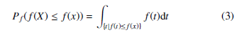
For a discrete variable, P_f (f(X) ≤ f(x)) is defined as the sum of all probabilities less than or equal to P_f (x), that is

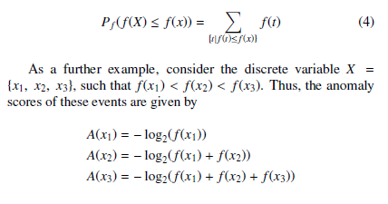
As a further example, consider the discrete variable X = {x₁, x₂, x₃}, such that f(x₁) < f(x₂) < f(x₃). Thus, the anomaly scores of these events are given by

A(x₁) = − log₂(f(x₁))

A(x₂) = − log₂(f(x₁) + f(x₂))

A(x₃) = − log₂(f(x₁) + f(x₂) + f(x₃))

In this case, it is clear that A(x₁) > A(x₂) > A(x₃); in other words, as the events become more common, they become less anomalous.

Bringing this to the scope of our work, the variables are the features we extract from the graph as described in subsection 5.2. Each feature is a multinomial variable with k categories, each defined by an n-tuple. For instance, the categories of feature totalsessions are defined by the 2-tuple (SourceHost, DestinationHost), whose values are defined by the total number of sessions between those hosts.

Now recall the importance of a suitable distribution for each variable. This is normally obtained through a training phase. However, because our model is fully unsupervised, it does not contain a training phase. Instead, we estimate the probability of each observed value online based on the frequency of that observation in the sample extracted from the graph, which collectively describe the probability mass function of the feature.

This implies that, although the values of each category of a variable might be continuous in theory, they are discrete in practice, which may cause some issues. Consider, for example, the following sample of a feature: {x₁ = 22, x₂ = 11, x₃ = 22, x₄ = 555, x₅ = 10, x₆ = 9}.

Intuitively, x₄ should have the higher anomaly score as its value is farther from the values of the others, but that is not the case. Instead, when considering the frequency of each value, x₁ and x₃ have the same values and thus the same higher probability (i.e. 2/6) and the same anomaly score. The other values, including the value for x₄, each appear only once and thus result in the same lower probability (i.e. 1/6) and the same anomaly score.

To overcome this issue, we discretize the values into bins such that neighbouring values will be mapped to the same bins and thus have a higher probability. In practice, given a bin width h, the binned value of x is defined as

Note that multiplying by h is only done to keep the binned values near to the original values but is not required in practice.

To help with understanding, Table 1 shows the binned values of a sample using different bin widths. The values with lower probabilities, meaning the most anomalous, for each bin width are bolded.

Table 1: Value binning examples 5

x1	22	20	0
x2	11	10	0
x3	22	20	0
x4	555	555	550
x5	10	10	0
x6	9	5	0

It can be seen that as the bin width increases, more similar values are mapped into the same bins, which increases their probabilities. With the bin width of 25, all values except that of x₄ are mapped to the same bin, resulting in a probability of 5/6, while x₄ continues to have a probability of 1/6, making it the most anomalous event in the sample for this bin width.

To compute the features, we first split the time range of the data into time windows, with the windows treated independently from each other. For that, we employed the previously discussed sliding window mechanism. Then, for each time window, we extract the features from the AEN graph.

Afterwards, for each feature X = {x₁, …, x_k} where k is the size or number of categories of X, its values are binned according to (5). After this process, there will be n bins, with each bin representing a value range. The probability of each bin, p(b_j), where j = {1, …, n}, is defined as the ratio of the number of elements in the bin over the total number of categories of the feature:

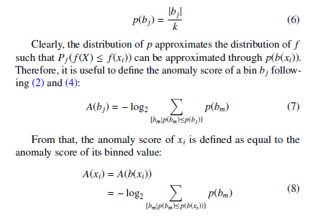
The last step of the anomaly detection is to compare the anomaly scores with a predefined threshold such that if the anomaly score of an element is greater than the threshold, that element is considered anomalous. Specifically, the source element of the anomalous feature tuples are the ones actually considered anomalous. For instance, for feature totalsessions, it is the source host, not the destination host, that is reported as anomalous.

5.2. Feature Model

In this subsection, we describe the proposed feature model, which contains a wide range of features extracted from the AEN graph.

The features are categorized into session features, which are extracted from session data, and authentication features, which are extracted from authentication data.

Note that all features are contained within a time window, meaning that each operation described below is performed only on the edges that were created in that time window. Also note that the features are directed, so any feature extracted for a pair of hosts h₁ and h₂ is different from that same feature between h₂ and h₁.

5.2.1       Session Features

The main type of edge in the AEN graph model is the session edge, which represents a communication session between two hosts. Our detection model leverages session edges to extract useful features that can support threat identification.

There are a total of nine session features:

• Total sessions: The total number of sessions between a pair of hosts.
• Unique destination ports: The number of unique ports of a destination host for which there are sessions from a source host.
• Unique destination hosts with same destination port: The number of unique destination hosts to which a source host connected with the same destination port. • Unique destination ports for a source host: The number of unique destination ports for which a host has sessions. • Mean time between sessions: The mean time between the start of the subsequent sessions between a pair of hosts. • Mean session duration: The mean duration of the sessions between a pair of hosts.
• Mean session size ratio: The mean ratio of the destination size (bytes sent from the destination host of the session) over the source size (bytes sent from the source host of the session) for a pair of hosts.
• Mean session velocity: The mean velocity of the sessions between a pair of hosts. The session velocity is defined as the ratio of the total number of packets of a session to the total duration of the session, which is expressed in packets/sec. • Mean session source size: The mean source size of the sessions sent from a host.

5.2.2       Authentication Features

The authentication data contained in the AEN graph are potential sources of useful information for the detection of anomalous authentication behaviour. There are a total of six different authentication features:

• Total authentication failures: The total number of failed authentication attempts between a pair of hosts. • Total authentication failures per account per host: The total number of failed authentication attempts by a host using a specific account to all other hosts.
• Total authentication failures per account: The total number of failed authentication attempts between a pair of hosts using a specific account.
• Unique accounts: The number of unique accounts that were used in failed authentication attempts between a pair of hosts. • Unique accounts per host: The number of unique accounts that were used in failed authentication attempts by a host to all other hosts.
• Unique target hosts per host per account: The total number of hosts that a host attempted, but failed, to authenticated using a specific account.

6. Experimental Evaluation

6.1. Setup and Procedures

The proposed ensemble intrusion detection mechanism was evaluated in two separate sets of experiments, one using the ISOT-CID Phase 1 dataset and one using the CIC-IDS2017 dataset. These datasets were selected because they contain benign and malicious network traffic data that can be used to build an AEN graph. Additionally, both datasets include examples of the attacks for which fingerprints have been developed, allowing their performance to be assessed.

The goal of the experiments was to evaluate the model’s performance in correctly classifying hosts as malicious or benign. Specifically, each of the two detection schemes were assessed individually, and afterwards, a final ensemble classification was performed.

Separate experiments were performed for each day of each of the datasets according to the following procedure: • An AEN graph was generated based on the available data of the specific day.

• Each of the two schemes were executed against the generated graph, and the results were collected.
• Each host node was given three classifications, one for each of the two detection schemes and one for the combined classification. The rules employed for each classifier are described later.
• The classification performance of each of the two individual schemes and that of the ensemble classifier were calculated based on the actual and predicted classifications.

The details for each of the two schemes are described in the following sections.

6.1.1       Fingerprint Matching

The fingerprint matching scheme classifies a host as malicious if the host is found to be part of an attack by at least one fingerprint.

Table 2 shows the parameters adopted for the experiment. Parameters with the same values used by multiple fingerprints are marked as “Multiple/Default”, while parameters that are unique to a single fingerprint or values that are distinct from the default are marked according to the fingerprint.

Table 2: Attack fingerprint experiment parameters

Fingerprint	Parameter	Value
Multiple/Default	attemptThr authFailRatioThr cntThr sessionThr	50 0.8 700 100
	sizeThr	600 bytes
	twSize	20 seconds
	twStep	10 seconds
Basic Pwd Guessing	attemptThr	4
Credential Stuffing	hostThr	4
HTTP Flood	pktCntThr sizeThr twSize	15000 1200 bytes 2 minutes
	twStep	1 minute
IP Fragmentation Attack	fragPckCntThr fragRatioThr	600 0.8
	sessionThr	20
Spraying Pwd Guessing	accountThr	4
TCP SYN Flood	synAckRatio	100
UDP Flood	sessionThr	300
Vertical Port Scanning	durThr portThr	1 second 50

Finally, to measure the performance of the fingerprints, we used precision (positive predicted value – PPV) and sensitivity (true positive rate – TPR) because they describe the detection performance of the scheme without taking into consideration the true negatives, which is desirable for evaluating the performance of a signaturebased intrusion detection scheme. Specifically, precision is better suited for the task because it describes the ratio of true positives among all predicted positive elements, which is expected to be high for a signature-based intrusion detection scheme. In contrast, sensitivity, indicates the ratio of true positives among all actual positive elements. This is not necessarily expected to be high given that the provided fingerprints only cover a few specific types of attacks and not all attack types that exist in the dataset.

6.1.2       Anomaly Detection

The anomaly detection scheme classifies a host as malicious if it is found to be the source of any anomalous behaviour, that is, if any of the features reports a score for the host above the experiment’s threshold.

The algorithm has four parameters, bin width, time window size, time window step and threshold. To assess the performance of the scheme under different combinations of parameters, and identify the optimal threshold value, we defined the following set of values:

• Bin width: 1, 2, 4, 12 and 64.
• Time window size: 30 minutes, 1 hour, 4 hours and 12 hours.
• Time window step: Half the time window size.
• Threshold: From 0 to 20 bits at 0.5 intervals.

As a consequence, for each day experiment, the anomaly detection was executed 20 times, once for each parameter combination (excluding the threshold). Afterwards, the scores were evaluated against the 40 thresholds, resulting in a total of 800 sets of results.

Finally, to measure the performance of the anomaly detection scheme, three metrics were chosen: F1 score, bookmaker informedness (BM), and the Matthews correlation coefficient (MCC). As discussed later, both datasets are unbalanced; therefore, traditional metrics like the accuracy, precision and recall were not suitable, and as such, they were not used for the evaluation. Conversely, the three chosen metrics, particularly the latter two, were chosen because they are generally considered to be better suited for this scenario [49, 50].

Nonetheless, we provide the resulting receiver operating characteristic (ROC) curve for each of the parameter combinations, representing the classifications of the separate days combined together, to show the general performance behaviour of the scheme under different parameters and different thresholds. This serves as a basis for selecting the best parameter combinations and, accordingly, discussing the performance of the algorithm. We also present the sensitivity and the false positive rate (1 − specificity) when discussing the performance of the best parameter combination so it can be correlated to the ROC curves.

6.1.3       Ensemble Classification

The ensemble classification was performed by fusing the classification of the individual schemes (classifiers) in two ways: One with an and rule, meaning a host is only considered malicious if both classifiers agree that it is malicious, and the other with an or rule, meaning that a host is considered malicious if either of the classifiers consider it malicious.

Naturally, the and rule is expected to generate few false positives and more false negatives. In contrast, the or rule is expected to generate more false positives and few false negatives. In practice, the classifier with fewer positive predictions sets an upper limit on those numbers when using the and rule and a lower limit when the or rule is applied.

6.2. ISOT-CID Phase 1

The ISOT-CID Phase 1 dataset [5] contains systems calls, system and event logs, memory dumps and network traffic (TCPdump) data extracted from Windows and Linux virtual machines (VMs) and OpenStack Hypervisors collected from a production cloud computing environment, more specifically, Compute Canada’s WestGrid. It includes both benign and malicious traces of several human generated attacks and of unsolicited Internet traffic.

The dataset includes the time stamps and IP addresses related to each attack, as well as the IP addresses that generated benign traffic. There is also a label file that labels each packet in the dataset’s network traffic data as benign or malicious, and the malicious packets are labelled by the type of attack. Unsolicited traffic is labelled as malicious but does not have an attack type label.

6.2.1       Graph Generation

In this study, we used only the network traffic data from which we extracted communication patterns between hosts, and system logs from which we extracted authentication information.

The graph elements are labelled based on the dataset labels, with host nodes labelled as malicious if they are the source of at least one packet labelled as malicious. The labels of other elements are derived from the host labels such that elements related to the host inherit its labels. For instance, a session edge is labelled as malicious if its source host is labelled as malicious. The malicious session edges are also labelled with the attack type when available. Note that labels are independent for each day of the data, meaning that they are not maintained from one day to the next.

The details of the generated AEN graphs for each day are shown in Table 3, and the sessions’ attack type labels are shown in Table 4. As can be seen in both tables, there is a high prevalence of malicious hosts and sessions; however, most malicious sessions are not labelled with an attack type. Moreover, each day has at least a few samples of different known types of attacks, but there were no samples of any DoS attacks.

Table 3: Graph details for ISOT-CID Phase 1 dataset

Day	Nodes	Hosts (malicious)	Edges	Sessions (malicious)
Day 1	376	78 (60 – 77%)	12432	8313 (7279 – 88%)
Day 2	635	134 (116 – 87%)	45334	17544 (14276 – 81%)
Day 3	653	86 (70 – 81%)	31405	9355 (8741 – 93%)
Day 4	491	94 (78 – 83%)	8258	4637 (3882 – 84%)
Combined	2155	392 (324 – 83%)	97429	39849 (34178 – 86%)

Table 4: Malicious session attack type labels for ISOT-CID Phase 1 dataset. PG stands for password guessing, PS for post scanning and UL for unauthorized login.

Day	PG	Ping	PS	UL	Unknown
Day 1	21	1	3	13	7241
Day 2	38	–	11	4	14223
Day 3	20	–	12	2	8707
Day 4	–	–	–	2	3880
Combined	79	1	26	21	34178

6.2.2       Fingerprint Matching Results

The results obtained after running the fingerprints on the generated graph for each of the four days of the dataset are shown in Tables 5 and 6, with the former showing the classification performance of the proposed fingerprints combined for each day and the latter showing the individual performance of each fingerprint. Fingerprints for which no matches were found are omitted.

Table 5: Classification performance of the proposed fingerprint matching scheme for ISOT-CID Phase 1 dataset

Day	TP	TN	FP	FN	PPV	TPR
Day 1	28	17	1	32	0.97	0.47
Day 2	24	18	0	92	1.00	0.21
Day 3	38	16	0	32	1.00	0.54
Day 4	23	16	0	55	1.00	0.29
Combined	113	67	1	211	0.99	0.35

As shown in Table 5, the fingerprints had very high precision for all days of the dataset with only a single false positive match resulting in a combined precision of over 0.99, which, as discussed previously, was expected given that the scheme is signature-based and given the high prevalence of malicious hosts in the dataset. The sensitivity was medium to low, depending on the day, which was once again expected, given the small number of attack types covered by the fingerprints.

Table 6: Individual fingerprint performance for ISOT-CID Phase 1 dataset. PG stands for password guessing. Fingerprints for which no matches were found are omitted.

TP            TP            TP            TP

       Basic PG             24       0       19       0       35       0       22       0

       Spraying PG       28       1       24       0       38       0       23       0

Looking at the performance of the individual fingerprints in

Table 6, we can see that there were only two fingerprints for which matches were found, namely the basic password guessing fingerprint and the spraying password guessing fingerprint. To understand the reason for that, we need to refer back to Table 4, where two notable pieces of information are shown. The first is that there are no known samples of DoS attacks in the dataset, which means that none of those fingerprints were expected to be matched. The second is that, while there were a few port scanning attacks, they involved a very small number of sessions (the maximum being 26 on day 4), which maps to a small number of ports scanned in total since each session only has one destination port. Moreover, as the dataset documentation states, these attacks were horizontal scans targeting only a few ports across several hosts in the network, while the available port scanning fingerprint is designed for vertical scans. Therefore, it was expected to find no matches for that fingerprint.

Note that it would be possible for samples of those attacks to be unknowingly present in the dataset from the collected unsolicited traffic. However, no instances of those attacks were observed, except for some instances of password guessing attacks.

Also of note is the fact that the network data in the dataset were sampled and thus contain gaps that can skew some of the graph elements. This can also explain some false negatives and even cause false positives.

6.2.3       Anomaly Detection Results

After running the experiments as previously described, the results from different days were combined, and an ROC curve was plotted for each of the parameter combinations. The curves are shown in Figure 2. Marked in each plot is the point where the threshold is equal to 0.5.

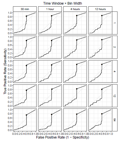
Figure 2: ROC curves of the anomaly detection scheme for the ISOT-CID Phase 1 dataset under different parameter combinations. The point in each plot marks where the threshold is equal to 0.5.

All curves show a similar pattern in which the sensitivity is poor while the threshold is high, until a point where it sharply rises until reaching its peak performance close to where the threshold is equal to 0.5. After that, it just goes straight to the top-right endpoint. Both of these characteristics can be explained by the exponential nature of the score, which means that a linear increase in the threshold will cause an exponential decrease in the true positives identified by the model. For this reason, it is common for the maximum score reported by any feature to be between 0 and 0.5, but the probability is exponentially smaller for higher scores.

When comparing the different ROC curves with regard to the other two parameters, a slightly better performance can be observed with longer time windows of 4 and 12 hours and with smaller bin widths of 1 and 2. That demonstrates that the extra information available with longer time windows allows the model to better distinguish anomalous behaviour. However, there is a limit to this, considering that too-long time windows could possibly be hiding shorter duration attacks. Also, the smaller bin widths allow for a greater variability of behaviours to be modelled. In practice, bin widths that are too large result in low resolutions of the distributions of variables that is caused by very diverse values being binned together.

These findings become even more clear when analyzing the other performance metrics, which are more suitable for the unbalanced nature of this dataset. Therefore, we selected a threshold of 0.5, bin width of 2 and time window size of 12 hours to discuss the findings further. Table 7 shows the daily and combined results of the model under that specific parameter combination.

Table 7: Performance of the proposed anomaly detection model for the ISOT-CID Phase 1 dataset

Day	TP	TN	FP	FN	TPR	FPR	F1	BM	MCC
Day 1	52	8	10	8	0.87	0.56	0.85	0.31	0.32
Day 2	94	7	11	22	0.81	0.61	0.85	0.20	0.16
Day 3	61	7	9	9	0.87	0.56	0.87	0.31	0.31
Day 4	71	7	9	7	0.91	0.56	0.90	0.35	0.37
Comb.	278	29	39	46	0.86	0.57	0.87	0.28	0.27

As can be seen, under the selected parameters, the model was able to detect the majority of the malicious hosts but also generated a relatively high number of false positives. That behaviour can be observed in the other metrics as well, with a combined F1-score of 0.87, a combined BM of 0.28 and a combined MCC of 0.27. Another notable aspect is the mostly consistent performance observed for each individual day, with only the results for day 2 having a greater deviation from the average.

In general, the observed behaviour was expected, given that the model is anomaly-based and thus prone to generating false alarms. Moreover, the high prevalence of hosts in the dataset means that the malicious behaviour is in fact not anomalous in the dataset. On the contrary, most of the traffic and hosts are labelled as malicious, which explains why the scheme generated a high number of false positives and points to a general limitation of anomaly-based detection, which can produce degraded results when the malicious behaviour is not uncommon.

6.2.4       Ensemble Classification Results

The ensemble classification using the and rule resulted in the same predictions as the fingerprint matching already shown in Table 5. This outcome means that all hosts classified as malicious by fingerprint matching were also classified as malicious with the anomaly detection. In contrast, but for the same reason, the ensemble classification using the or rule resulted in the same predictions as the as anomaly detection, which are summarized in Table 7.

In practice, in a real environment, where the anomaly detection threshold is not optimally chosen, the divergence between the classifiers will be greater, thus causing the performance of the ensemble classification to be distinct. Other ensemble classification rules, such as soft voting could also be used as a middle ground between the two rules evaluated in this paper.

6.3. CIC-IDS2017

The CIC-IDS2017 dataset [6] contains network traffic data (both pcap and NetFlow) of benign traffic, as well as several samples of attack scenarios including SSH and FTP password guessing, DoS, web attacks and instances of host infiltration. The dataset is labelled on the flow level, with each flow being labelled as either benign or with the attack performed.

6.3.1       Graph Generation

To build the graph, the packet data (pcap files) were used to extract the communication patterns between hosts since packets are more finely detailed than flow data. Because no system or application logs were available, we could not extract authentication information from the data. As a consequence, no authentication-related elements (account nodes and authentication attempt edges) are present in the graphs of this dataset which in turn means that no password guessing instances can be found with the fingerprints as designed.

The graph labelling followed the same rules as the previous dataset, with host nodes labelled as malicious if they were the source of at least one flow labelled as malicious and with the labels of other elements being derived from the host labels. One distinction was how to define the attack type labels. For that, we first combined the dataset labels into generic attack type labels. For instance, the “DoS slowloris” and “DoS GoldenEye” labels were combined into the “Denial of Service” label. Then, each flow was matched with its respective session edge that was labelled with the generic attack type.

In a few cases, sessions had more than one attack type. This was an artifact of how the sessions are created from packets such that one session can map to more than one flow. Moreover, some malicious sessions have no attack type labels in cases where none of their mapped flows were labelled as malicious, even though their source hosts were labelled as such.

The details of the generated AEN graphs for each day are shown in Table 8, and the sessions’ attack type labels are shown in Table 9. As shown by the tables, there was a very small prevalence of malicious hosts, while the prevalence of malicious sessions varied from low (approximately 3% on day 1) to high (approximately 87% on day 4). As for the attack type labels, there was a high number of attack samples from all days. However, the types of attacks present for each day varied with most types of attacks only present for one day. Moreover, the number of sessions with unknown attack was high on days 3 and 4, which stems from the fact that those days had combined multiple attack sessions.

Table 8: Graph details for the CIC-IDS2017 dataset

Day	Nodes	Hosts (malicious)	Edges	Sessions (malicious)
Day 1	27653	8498 (1 – 0.01%)	279271	243264 (6954 – 3%)
Day 2	29216	9017 (1 – 0.01%)	298033	259938 (16571 – 6%)
Day 3	27828	8545 (2 – 0.02%)	323502	287272 (89523 – 31%)
Day 4	27035	8331 (10 – 0.12%)	460893	425649 (370297 – 87%)
Comb.	111732	34391 (14 – 0.04%)	1361699	1216123 (483345 – 40%)

Table 9: Malicious session attack type labels for CIC-IDS2017 dataset. BN stands for botnet, Inf for infiltration, PG for password guessing, PS for port scanning, WA for web attack and Unk for unknown.

Day	BN	DoS	Inf	PG	PS	WA	Unk
Day 1	–	–	–	6953	–	–	1
Day 2	–	16537	1	–	–	–	33
Day 3	–	–	6	1363	–	643	87511
Day 4	1228	45392	–	–	158678	–	165026
Comb.	1228	61929	7	8316	158678	643	252571

6.3.2       Fingerprint Matching Results

The results obtained after running the fingerprints on the generated graph for each of the four days of the dataset are shown in Tables 10 and 11, with the former table showing the classification performance of the proposed fingerprints combined for each day and the latter showing the individual performance of each fingerprint. Fingerprints for which no matches were found are omitted.

Table 10: Classification performance of the proposed fingerprints for the CICIDS2017 dataset

Day	TP	TN	FP	FN	PPV	TPR
Day 1	0	8494	3	1	0.00	0.00
Day 2	0	9011	5	1	0.00	0.00
Day 3	2	8542	1	0	0.67	1.00
Day 4	6	8320	1	4	0.86	0.60
Combined	8	34367	10	6	0.44	0.57

Table 11: Individual fingerprint performance for the CIC-IDS2017 dataset. PS stands for port scanning. Fingerprints for which no matches were found are omitted.

HTTP Flood	0	0	0	0	0	0	1	0
TCP SYN Flood	0	0	0	0	2	0	1	0
UDP Flood	0	1	0	2	0	0	1	0
Vertical PS	0	2	0	4	2	1	5	1

As shown in Table 10, the general performance was not as high as with the previous dataset. There were no true positive matches on days 1 and 2, resulting is precision and sensitivity of 0 for those days. In contrast, days 3 and 4 had better performance, particularly day 4, with a precision of 0.86.

Having no true positives was expected for day 1 because this day only had password guessing attacks but graph had no authentication elements, which are part of the password guessing fingerprints. This was not the case for day 2, which had DoS attacks that were HTTPbased, but no matches were found for the HTTP flood fingerprint. Still, this can be explained by the types of attacks performed, such as Heartbleed and Slowloris, which are not flood attacks, making the HTTP flood fingerprint unsuitable for this case. Tuning the fingerprint parameters might allow for these attacks to be found but might also result in some false positives. Moreover, the very low prevalence of malicious hosts, with only a single one for both days 1 and 2, means that not finding that host will result in a precision and sensitivity of 0 as observed.

Continuing onto day 3, there were matches for the two malicious hosts for both the TCP SYN flood fingerprint and the vertical port scanning fingerprint. Note that according to the dataset labels, as shown in Table 9, neither type of attack was expected to be present. However, the dataset documentation states that both port scans and nmap scans were performed on that day, although not labelled, which explains the positive matches.

As for day 4, there were matches for four different fingerprints, including three DoS fingerprints and the port scanning fingerprint. The day’s data are labelled as having both of those types of attacks, as well as a botnet attack. Sessions with all three labels were matched. Note that the dataset’s documentation is not clear on exactly which attacks were executed as part of the botnet attack, but in any case, the attack’s data were the source of some of the matches, too.

Finally, all days had false positives, which would not be expected from a signature-based scheme; however, the absolute number of false positives was low compared to the total number of hosts in the dataset. Moreover, as shown in Table 11, this was mostly from the vertical port scanning fingerprint. When analyzing the benign sessions that were matched by that fingerprint, almost 60% had port UDP/137, which is used by the NetBIOS name service. However, in these cases, it was not the destination port that was fixed at 137, but instead, the source port was 137, while the destination port varied. This behaviour is an artifact of how name queries are broadcast in NetBIOS, but the replies are directed to the host that made the query on what was originally the source port of the broadcast query. The rest of the false positives do not have such a clear explanation. Tuning the fingerprint parameters could reduce them but would also reduce the detection rate.

6.3.3       Anomaly Detection Results

After running the experiments as previously described, the results from different days were combined, and an ROC curve was plotted for each of the parameter combinations. The curves are shown in Figure 3. Marked in each plot is the point where the threshold is equal to 0.5.

All parameter combinations showed high levels of performance, with an area under the ROC curve (AUC) of over 0.99. However, that metric by itself is deceiving, given the highly unbalanced nature of the dataset. In reality, the model was able to detect all 14 malicious hosts with thresholds between 0.5 to 5.5 under most parameter configurations, but it reported a decreasing number of false positives as the threshold increased. Nonetheless, the relative variation was small in terms of the total number of benign hosts in the dataset.

Although not distinguishable from the ROC curves, the behaviour observed for the previous dataset with regards to the bin width can also be observed for this dataset when analyzing the other metrics, with values of 1 and 2 resulting in a better performance on average than the others. However, the benefit of a longer time window parameter is not as clear for this dataset, which shows a more mixed performance with different values for this parameter.

Based on that, we selected a threshold of 5, bin width of 1 and time window size of 12 hours for further discussion. Table 12 shows the daily and combined results of the model under that specific parameter combination.

Figure 3: ROC curves of proposed scheme under different parameter combinations for the CIC-IDS2017 dataset. The point in each plot marks where the threshold is equal to 0.5.

Table 12: Performance of the proposed anomaly detection model for the CIC-

IDS2017 dataset

Day	TP	TN	FP	FN	TPR	FPR	F1	BM	MCC
Day 1	1	8481	16	0	1.00	0.01	0.11	0.99	0.24
Day 2	1	9001	15	0	1.00	0.01	0.12	0.99	0.25
Day 3	2	8529	14	0	1.00	0.01	0.22	0.99	0.35
Day 4	10	8313	8	0	1.00	0.01	0.71	0.99	0.75
Comb.	14	34324	53	0	1.00	0.01	0.34	0.99	0.46

As can be seen, under the selected parameters, the model was able to detect all malicious hosts in all days with a relatively low number of false positives. As a point of comparison, using the same parameters as the previous dataset (threshold of 0.5 and bin width of 2) would not affect the number of true positives but would result in an extra 145 false positives and only slightly worse performance.

Because of the very small prevalence of malicious hosts in the dataset, the observed performance resulted in a low F1-score and a medium MCC for all days except day 4, which had a higher number of malicious hosts that can compensate for the false positives.

Conversely, the BM was above 0.99 for all four days. In summary, the scheme obtained very good results for this dataset with a varied number of parameter configurations. This shows that the scheme is suitable for detecting malicious behaviour when the prevalence of malicious hosts is low and, therefore anomalous.

6.3.4       Ensemble Classification Results

As with the previous dataset, the ensemble classification using the and rule resulted in the same predictions as the fingerprint matching shown in Table 10, while the the ensemble classification using the or rule resulted in the same predictions as the anomaly detection.

These are summarized in Table 12. This again shows that hosts that were classified as malicious by fingerprint matching were also classified as malicious with the anomaly detection.

7. Conclusion

This paper presented an unsupervised ensemble intrusion detection mechanism composed of two detection schemes, one signature based that employs isomorphic subgraph matching of graphical patterns of known attacks, called attack fingerprints, and one anomaly based, which consists of an anomaly score developed based on the work of Farragut et al. [4].

To validate the proposed scheme we presented a collection of attack fingerprints for the AEN graph model, which were expressed using PGQL and covered common attacks, such as port scanning, DoS and password guessing, along with a subgraph matching algorithm specific for finding subgraphs isomorphic to the fingerprints. Furthermore, a total of 15 anomaly features, including nine extracted from session data and six extracted from authentication data.

The proposed schemes were evaluated individually and as an ensemble in the capacity for identifying malicious hosts using two datasets: The ISOT-CID Phase 1 dataset and the CIC-IDS2017 dataset.

The evaluation of the fingerprint matching scheme showed a combined precision of 0.99 and a combined sensitivity of 0.35 for the former dataset, while the latter dataset resulted in a combined precision of 0.44 and a combined sensitivity of 0.57. The observed results are promising, particularly considering the limited number of fingerprints available and the specific types of errors encountered. Ultimately, they demonstrate that the method is capable of identifying known attacks and is particularly suited to identifying stealth attacks, which is a weakness of traditional signature-based intrusion detection systems.

The evaluation of the anomaly detection was particularly encouraging for the CIC-IDS2017 dataset, with a BM of over 0.99 and an MCC of 0.46. This shows that the scheme has a high capacity for detecting anomalous behavior when there was a low prevalence of malicious elements in the network.

The evaluation of the ensemble classification showed that one classifier could end up dominating the ensemble classification. This underscores the need for future exploration of possible benefits from using ensemble classification rules, such as soft voting.

As limitations, we identified the amount of effort needed to create the fingerprints, the binning of the values anomaly features that can result in suboptimal distributions and the high computational power required to build and maintain the graph. Another limitation is the high computation cost involved in searching for isomorphic subgraphs given the high complexity of the subgraph matching algorithms, although the use of indexes helps alleviate that issue with the cost of extra memory requirements.

In our future work, we aim to improve and extend the proposed fingerprint database to add other types of attacks, particularly those that are traditionally harder to detect, such as HTTP request smuggling, and to increase the feature space of the anomaly detection model by introducing more features. We believe this can help improve detection accuracy, particularly in environments that have a high prevalence of malicious hosts.

We also plan to implement more advanced classification rules as part of the anomaly detection scheme and also in the ensemble classification of the two detection schemes. In addition, we plan to employ adaptive bin width values according to the value range of each given variable to improve the fitness of the bin distributions.

Finally, we aim to conduct further evaluations using other datasets, such as the ISOT-CID Phase 2 dataset and the 2018 CIC Intrusion Detection Evaluation Dataset (CSE-CIC-IDS2018) [51].

1. C. Nie, P. G. Quinan, I. Traore´, I. Woungang, “Intrusion Detection using a Graphical Fingerprint Model,” in 2022 22nd IEEE International Sympo- sium on Cluster, Cloud and Internet Computing (CCGrid), 806–813, 2022, doi:10.1109/CCGrid54584.2022.00095.
2. R. Sommer, V. Paxson, “Outside the Closed World: On Using Machine Learn- ing for Network Intrusion Detection,” in Proceedings of the 2010 IEEE Sym- posium on Security and Privacy, SP ’10, 305–316, IEEE Computer Society, Washington, DC, USA, 2010, doi:10.1109/SP.2010.25.
3. A. Aldribi, I. Traore´, B. Moa, O. Nwamuo, “Hypervisor-based cloud intrusion detection through online multivariate statistical change tracking,” Computers & Security, 88, 2020, doi:10.1016/j.cose.2019.101646.
4. E. M. Ferragut, J. A. Laska, R. A. Bridges, “A New, Principled Approach to Anomaly Detection,” 2012 11th International Conference on Machine Learning and Applications, 2, 210–215, 2012, doi:10.1109/ICMLA.2012.151.
5. A. Aldribi, I. Traore, B. Moa, Data Sources and Datasets for Cloud Intrusion Detection Modeling and Evaluation, 333–366, Springer International Publish- ing, Cham, 2018, doi:10.1007/978-3-319-73676-1 13.
6. I. Sharafaldin, A. H. Lashkari, A. A. Ghorbani, “Toward generating a new intrusion detection dataset and intrusion traffic characterization.” in ICISSP, 108–116, 2018, doi:10.5220/0006639801080116.
7. C. Phillips, L. P. Swiler, “A Graph-based System for Network-vulnerability Analysis,” in Proceedings of the 1998 Workshop on New Security Paradigms, NSPW ’98, 71–79, ACM, New York, NY, USA, 1998, doi:10.1145/310889. 310919.
8. O. Sheyner, S. Haines, Jand Jha, R. Lippmann, J. M. Wing, “Automated gen- eration and analysis of attack graphs,” in Proceedings of the Symposium on Security and Privacy, IEEE, 2002, doi:10.1109/SECPRI.2002.1004377.
9. S. Jha, O. Sheyner, J. Wing, “Two formal analyses of attack graphs,” in Pro- ceedings 15th IEEE Computer Security Foundations Workshop. CSFW-15, 49–63, 2002, doi:10.1109/CSFW.2002.1021806.
10. X. Ou, G. Sudhakar, A. A. W., “MulVAL: A Logic-based Network Security Analyzer,” in Proceedings of USENIX Security Symposium, volume 8, 2005, doi:10.5555/1251398.1251406.
11. K. Ingols, R. Lippmann, K. Piwowarski, “Practical Attack Graph Generation for Network Defense,” in 2006 22nd Annual Computer Security Applications Conference (ACSAC’06), 121–130, 2006, doi:10.1109/ACSAC.2006.39.
12. L. Akoglu, H. Tong, K. D., “Graph based Anomaly Detection and Description: A Survey,” Journal Data Mining and Knowledge Discovery, 29(3), 626–688,
    2015, doi:10.1007/s10618-014-0365-y.
13. F. Jemili, M. Zaghdoud, M. B. Ahmed, “Intrusion detection based on “Hybrid” propagation in Bayesian Networks,” 2009 IEEE International Conference on Intelligence and Security Informatics, 137–142, 2009, doi:10.1109/ISI.2009. 5137285.
14. P. Xie, J. H. Li, X. Ou, P. Liu, R. Levy, “Using Bayesian networks for cyber security analysis,” 2010 IEEE/IFIP International Conference on Dependable Systems & Networks (DSN), 211–220, 2010, doi:10.1109/DSN.2010.5544924.
15. L. Xiao, Y. Chen, C. K. Chang, “Bayesian Model Averaging of Bayesian Network Classifiers for Intrusion Detection,” 2014 IEEE 38th International Computer Software and Applications Conference Workshops, 128–133, 2014, doi:10.1109/COMPSACW.2014.25.
16. K. K. Gupta, B. Nath, K. Ramamohanarao, “Conditional Random Fields for In- trusion Detection,” in 21st International Conference on Advanced Information Networking and Applications Workshops (AINAW’07), volume 1, 203–208, IEEE, 2007, doi:10.1109/AINAW.2007.126.
17. H. Ma, Y. Xie, S. Tang, J. Hu, X. Liu, “Threat-Event Detection for Dis- tributed Networks Based on Spatiotemporal Markov Random Field,” IEEE Transactions on Dependable and Secure Computing, 19(3), 1735–1752, 2022, doi:10.1109/TDSC.2020.3036664.
18. K. Peng, V. C. M. Leung, L. Zheng, S. Wang, C. Huang, T. Lin, “Intrusion Detection System Based on Decision Tree over Big Data in Fog Environ- ment,” Wireless Communication and Mobile Computing, 2018, 2018, doi: 10.1155/2018/4680867.
19. C. Yin, Y. Zhu, J. long Fei, X.-Z. He, “A Deep Learning Approach for Intrusion Detection Using Recurrent Neural Networks,” IEEE Access, 5, 21954–21961, 2017, doi:10.1109/ACCESS.2017.2762418.
20. Y. Zhang, P. Li, X. Wang, “Intrusion Detection for IoT Based on Improved Genetic Algorithm and Deep Belief Network,” IEEE Access, 7, 31711–31722, 2019, doi:10.1109/ACCESS.2019.2903723.
21. Z. Wang, Y. Zeng, Y. Liu, D. Li, “Deep Belief Network Integrating Improved Kernel-Based Extreme Learning Machine for Network Intrusion Detection,” IEEE Access, 9, 16062–16091, 2021, doi:10.1109/ACCESS.2021.3051074.
22. S. A. Cook, “The complexity of theorem-proving procedures,” in Proceedings of the third annual ACM symposium on Theory of computing, 151–158, 1971, doi:10.1145/800157.805047.
23. J. E. Hopcroft, J.-K. Wong, “Linear time algorithm for isomorphism of planar graphs (Preliminary Report),” in Proceedings of the sixth annual ACM sympo- sium on Theory of computing, 172–184, 1974, doi:10.1145/800119.803896.
24. J. R. Ullmann, “An algorithm for subgraph isomorphism,” Journal of the ACM (JACM), 23(1), 31–42, 1976, doi:10.1145/321921.321925.
25. L. P. Cordella, P. Foggia, C. Sansone, M. Vento, “A (sub)graph isomorphism algorithm for matching large graphs,” IEEE Transactions on Pattern Analysis and Machine Intelligence, 26, 1367–1372, 2004, doi:10.1109/TPAMI.2004.75.
26. W.-S. Han, J. Lee, J.-H. Lee, “Turboiso: towards ultrafast and robust sub- graph isomorphism search in large graph databases,” in SIGMOD ’13, 2013, doi:10.1145/2463676.2465300.
27. M. Han, H. Kim, G. Gu, K. Park, W.-S. Han, “Efficient Subgraph Match- ing: Harmonizing Dynamic Programming, Adaptive Matching Order, and Failing Set Together,” Proceedings of the 2019 International Conference on Management of Data, 2019, doi:10.1145/3299869.3319880.
28. P. G. Quinan, I. Traore´, I. Woungang, “Activity and Event Network Graph and Application to Cyberphysical Security,” in I. Traore´, I. Woungang, S. Saad, edi- tors, Artificial Intelligence for Cyber-Physical Systems Hardening, chapter 10, 217–233, Springer, 2022, doi:10.1007/978-3-031-16237-4 10.
29. O. van Rest, S. Hong, J. Kim, X. Meng, H. Chafi, “PGQL: a property graph query language,” in GRADES ’16, 2016, doi:10.1145/2960414.2960421.
30. N. Francis, A. Green, P. Guagliardo, L. Libkin, T. Lindaaker, V. Marsault, S. Plantikow, M. Rydberg, P. Selmer, A. Taylor, “Cypher: An Evolving Query Language for Property Graphs,” Proceedings of the 2018 International Conference on Management of Data, 2018, doi:10.1145/3183713.3190657.
31. M. H. Bhuyan, D. K. Bhattacharyya, J. K. Kalita, “Surveying Port Scans and Their Detection Methodologies,” The Computer Journal, 54, 1565–1581, 2011, doi:10.1093/comjnl/bxr035.
32. S. Staniford, J. A. Hoagland, J. M. McAlerney, “Practical Automated Detec- tion of Stealthy Portscans,” Journal of Computer Security, 10, 105–136, 2002, doi:10.3233/JCS-2002-101-205.
33. M. De Vivo, E. Carrasco, G. Isern, G. O. de Vivo, “A review of port scan- ning techniques,” ACM SIGCOMM Computer Communication Review, 29(2), 41–48, 1999, doi:10.1145/505733.505737.
34. J. Mirkovic, P. L. Reiher, “A taxonomy of DDoS attack and DDoS defense mechanisms,” Comput. Commun. Rev., 34, 39–53, 2004, doi:10.1145/997150. 997156.
35. R. Tandon, “A Survey of Distributed Denial of Service Attacks and Defenses,” ArXiv, abs/2008.01345, 2020, doi:10.48550/arXiv.2008.01345.
36. E. Cambiaso, G. Papaleo, G. Chiola, M. Aiello, “Slow DoS attacks: definition and categorisation,” International Journal Trust Management in Computing and Communications, 1, 300–319, 2013, doi:10.1504/IJTMCC.2013.056440.
37. M. Bogdanoski, T. Suminoski, A. Risteski, “Analysis of the SYN flood DoS attack,” International Journal of Computer Network and Information Security (IJCNIS), 5(8), 1–11, 2013, doi:10.5815/IJCNIS.2013.08.01.
38. V. K. Yadav, M. C. Trivedi, B. Mehtre, “DDA: an approach to handle DDoS (Ping flood) attack,” in Proceedings of International Conference on ICT for Sustainable Development, 11–23, Springer, 2016, doi:10.1007/ 978-981-10-0129-1 2.
39. T. H. Ptacek, T. N. Newsham, “Insertion, Evasion, and Denial of Service: Eluding Network Intrusion Detection,” Technical report, Secure Networks inc Calgary Alberta, 1998.
40. “Transmission Control Protocol,” RFC 793, 1981, doi:10.17487/RFC0793.
41. MazeBolt, “Layer 4 — MazeBolt Knowledge Base,” .
42. A. Bijalwan, M. Wazid, E. S. Pilli, R. C. Joshi, “Forensics of random-UDP flooding attacks,” Journal of Networks, 10(5), 287, 2015, doi:10.4304/jnw.10. 5.287-293.
43. I. Sreeram, V. P. K. Vuppala, “HTTP flood attack detection in application layer using machine learning metrics and bio inspired bat algorithm,” Applied Computing and Informatics, 2019, doi:10.1016/j.aci.2017.10.003.
44. C. Paar, J. Pelzl, B. Preneel, “Understanding Cryptography: A Textbook for Students and Practitioners,” 2010, doi:10.1007/978-3-642-04101-3.
45. D. Wang, Z. Zhang, P. Wang, J. Yan, X. Huang, “Targeted online password guessing: An underestimated threat,” in Proceedings of the 2016 ACM SIGSAC conference on computer and communications security, 1242–1254, 2016, doi: 10.1145/2976749.2978339.
46. Mitre, “Brute Force: Password Spraying,” .
47. M. Patton, E. Gross, R. Chinn, S. Forbis, L. Walker, H. Chen, “Uninvited connections: a study of vulnerable devices on the internet of things (IoT),” in 2014 IEEE joint intelligence and security informatics conference, 232–235, IEEE, 2014, doi:10.1109/JISIC.2014.43.
48. G. Tandon, P. K. Chan, “Tracking user mobility to detect suspicious behavior,” in Proceedings of the 2009 SIAM International Conference on Data Mining, 871–882, SIAM, 2009, doi:10.1137/1.9781611972795.75.
49. A. Luque, A. Carrasco, A. Mart´ın, A. de las Heras, “The impact of class imbal- ance in classification performance metrics based on the binary confusion ma- trix,” Pattern Recognit., 91, 216–231, 2019, doi:10.1016/j.patcog.2019.02.023.
50. D. Chicco, G. Jurman, “The advantages of the Matthews correlation coefficient (MCC) over F1 score and accuracy in binary classification evaluation,” BMC Genomics, 21, 2020, doi:10.1186/s12864-019-6413-7.
51. Canadian Institute for Cybersecurity, “CSE-CIC-IDS2018 on AWS: A collabo- rative project between the Communications Security Establishment (CSE) & the Canadian Institute for Cybersecurity (CIC),” .

(Click Here)