1. Introduction

Worldwide, 10 to 40% of crops die due to pests and diseases [1]. This issue will only get worse in the future, as temperature changes due to climate change will lead to more favorable conditions for pathogens [2]. In order to deal with this growing issue, it is necessary to come up with accurate diagnostic methods in order to quickly treat diseased plants. Focusing on maize, one of the most important crops in the world that accounts for two-thirds of the total volume of coarse grain trade globally in the past decade [3], in recent years, both Northern corn leaf blight, i.e., NLB, and Gray leaf spot disease has become more prevalent. In 2015, NLB was ranked first in most destructive corn disease in the northern United States and Ontario, Canada, up from seventh in 2012, with an estimated loss of 548 million bushels. For comparison, in 2015, the second-ranked most destructive corn disease, anthracnose stalk rot, had an estimated loss of 233 million bushels, less than half of NLB. In 2012, Gray leaf spot was ranked sixth in most destructive corn disease and has maintained its place as one of the top four most destructive from 2013-2015 [4]. NLB is caused by the fungus Exserohilum turcium, and the most distinguishing visual symptom of the disease is a cigar-shaped, tan lesion that can range from one to seven inches long, as shown in Figure 1. Gray leaf spot is a fungal disease caused by Cercospora zeae-maydis with rectangular lesions from two to three inches long, as shown in Figure 2., often leading to confusion by farmers due to its similarity to NLB lesions. Although fungicides can be used as a treatment for these two diseases, studies have shown that fungicides persist in aquatic systems and are toxic to organisms [5]. Early detection can mitigate the necessity of fungicides, traditionally through manual scouting [6]. However, this method is time-consuming and can result in inaccurate or missed diagnoses due to human error. As a result, several types of image-based machine learning solutions, such as convolutional neural networks, i.e., CNN, and object detection algorithms, have been proposed.

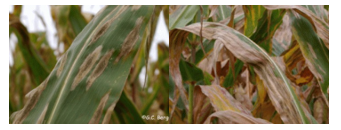
Figure 1: NLB infected maize images from Cornell CALS

CNNs are commonly used for image classification, which involves assigning an entire image to a single class label. However, in cases where the location of objects in an image is important, image classification can be difficult to interpret and verify. Object detection algorithms, on the other hand, can identify the specific location and extent of objects in an image, and can even draw bounding boxes around them to highlight their location. These algorithms can be useful in situations such as identifying disease symptoms in natural environment images, where it is important to know the exact location of the symptom. The typical symptoms of NLB and Gray leaf spot, which are brown, oval lesions, can be difficult to distinguish with the naked eye, but computer vision algorithms may be able to identify and differentiate them.

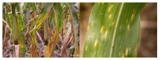
Figure 2: Gray leaf spot infected maize images from Cornell CALS

Many different object detection algorithms have been created, such as YOLOv3, which is both accurate and has low inference speed. Low inference speed is essential to speed up traditional manual practices and increases the likelihood of detecting a lesion on live video. However, one of the tradeoffs for its high inference speed is reduced accuracy. As a result, an optimized algorithm based on YOLOv3 was proposed in this paper by applying two methods: Dense blocks and convolutional block attention modules, i.e., CBAM. These optimizations were chosen to increase accuracy while maintaining or reducing inference speed compared to the base YOLOv3. In addition to proposing an improved algorithm, one of the main challenges of object detection is the need for more high-quality datasets, especially in niche areas such as plant disease detection. It is much easier to create image classification datasets because the label for an entire image is a single class or word. For object detection datasets, each image may contain more than one class, numerous objects per class, and requires the tedious work of locating all objects in an image and drawing bounding box labels around them. As a result, if there are no object detection datasets for a specific class, datasets originally for CNNs may be used instead by converting them to the correct format. In summary, this paper offers   the following contributions:

• Application of machine learning to detect NLB and gray leaf spot lesions
• An optimized YOLOv3 with improved detection ability without significantly increased inference speed
• A NLB and grey spot dataset suited for object detection

This paper is an extension of work originally presented in  IEEE 12th Annual Computing and Communication Workshop and Conference (CCWC) [7], and the paper is structured as follows: Section 2 is the related works. Section 3 explains the YOLOv3 model and its optimizations. Section 4 shows how the dataset was created and explains the evaluation metrics. Section 5 shows the performance of the algorithms, and section 6 is the conclusion.

2. Related Works

 Both image classification algorithms, such as CNNs and object detection algorithms, have been successfully applied for plant disease diagnosis. In [8], the authors used a CNN for plant disease diagnosis, training it on an extensive image dataset of close-up, individual diseased leaves using the Plant Village dataset. The dataset consists of images of twenty-six diseases of plants, such as those that affect corn and apple. They reported 99.35% accuracy on a held-out test set. However, the images in the dataset were taken in a lab environment, where variables such as the presence of multiple leaves in an image, orientation, brightness, and soil presence are not considered. Solving this issue, high-quality datasets have been created by experts.  In [9], the authors took images of NLB-infected corn and annotated each lesion individually with line annotations, which is the same dataset used in this paper. Because the images covered a large area, the actual lesions took up a small portion of the overall image. As a result, using a CNN on scaled-down versions of the images resulted in 70% accuracy. It was only after dividing the image into grids and associating a diseased-or-not class to each grid using their line annotations that resulted in 97.8% accuracy. Although successful, the process of dividing the image and then running inferences finally resulting in a high accuracy indicates a potential limitation of CNNs – they are not suited when the characteristics that define a class are small compared to the entire image.

On the other hand, object detection algorithms are suited to looking for specific areas in an image. The single shot detector, i.e., SSD [10] object detection algorithm, was used to detect apple diseases such as Brown Spot and Grey spot [11]. Instead of labeling an entire infected leaf as belonging to a class, the author only labeled the specific symptoms, such as spots, allowing the SSD algorithm to learn that the presence of a particular cluster of pixels determines the final output. The YOLOv3 [12] object detection algorithm was used to locate characteristics of various tomato diseases, such as early blight and mosaic disease [13]. The authors collected their own tomato dataset and annotated them by grouping clusters of diseased symptoms. In [14], the authors used a variant of an SSD and the Faster R-CNN [15] algorithm for grape plant disease object detection. They used existing datasets such as the Plant Village dataset, which mentioned previously is used for CNN training, drew boxes around the grape disease, converting it for object detection use. However, instead of drawing boxes around the grape disease symptoms, they label the entire leaf containing the disease, meaning it could be more specific. In [16], the authors also annotated the Plant Village dataset with bounding boxes for object detection. Instead of limiting to only certain disease classes, the entire dataset was used, resulting in about 54,000 annotated images. In [17], the authors created their object detection dataset called PlantDoc, which includes corn diseases, including both NLB and gray leaf spot. However, the dataset is small, less than 200 images per class, and the annotations are not very specific – clusters of lesions are grouped. This leads to the additional problem of determining whether two lesions belong to the same or different clusters, especially in images where lesions make up most of the corn leaf.

3. Methods

In this section, deep learning methods such as the usage of dense blocks, CBAM, and the proposed optimized algorithm to detect corn disease will be introduced.

3.1.  Base Algorithm: YOLOv3

YOLOv3 is an object detection algorithm that boasts high accuracy without sacrificing speed. It is an improvement of YOLO in 2016 [18] and YOLOv2 in 2017 [19]. Although newer variants exist, such as YOLOv4 [20], for this study, YOLOv3 was chosen as the algorithm to focus on because there is many open source code for the algorithm, meaning it was easier to find a repo with an implementation that could easily be modified. Also, YOLOv3, as shown in Figure 3, uses the darknet-53 backbone to extract features of images. The backbone network utilizes residual blocks containing skip connections, which was introduced in ResNet [21]. These skip connections skip some layers in the backbone, helping to alleviate the vanishing gradient problem and making it easier to tune the earlier layers of a network. In the figure, the residual N blocks consist of a 3×3 convolutional layer and N residual units. The detection stages contain additional convolutional layers for further feature extraction and detect potential objects on three different scales. These scales are used to detect large, medium, and small-sized objects. This improves the performance of varying image sizes. According to the YOLOv3 paper, performance on the Microsoft Common Objects in Context, i.e., MS COCO, dataset, a benchmark used for evaluating object detection algorithms in which the accuracy metric mean average precision, i.e., mAP, is commonly used, showed that the three fastest were YOLOv3-320, SSD321, and DSSD321 [22] with 51.5 mAP-50/22 ms, 45.4 mAP-50/61 ms, and 46.1 mAP-50/85 ms, respectively, indicating mAP and inference time. Compared to the other algorithms, YOLOv3 is significantly faster while achieving better mAP. As a result, YOLOv3 was selected as the base algorithm of our research because efficiency is critical for searching through large cornfields.

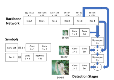
Figure 3: YOLOv3 diagram

 Dense Block

DenseNet [23] is a convolutional neural network architecture that uses dense blocks, in which the output of each convolution layer is connected to the inputs of all subsequent layers. This allows later layers to use information learned in earlier layers and reduces the number of parameters, improving computational efficiency and mitigating the vanishing gradient problem. Transition layers, which consist of a 1×1 convolution and average pooling layer, are placed between groups of dense blocks to reduce the number of parameters and dimensionality. The growth rate, denoted by k, determines the number of new feature maps added for each layer in a dense block.

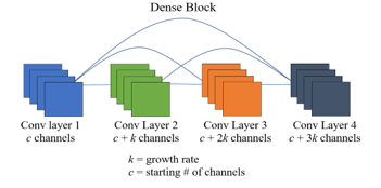
Figure 4: Diagram of 4 layer dense block

3.2.  CBAM

CBAM [24] is a method that uses the attention mechanism to replicate how humans pay attention to their environment. It uses both channel and spatial attention to focus on particular objects in a scene and enhance the feature maps of the convolutional layers. Channel attention selects the most important channels and weighs them to improve them, while spatial attention applies max pooling and average pooling to help the model know where to focus in the image. Using this method leads to improved accuracy with only a limited amount of extra computation.

3.3.  Proposed Algorithm

The proposed algorithm for an input image of 512×512 pixels is shown in Figure 5. The algorithm includes changes to the base YOLOv3 model, indicated by the yellow and green shaded portions. After the third residual block, a four-layer dense block is inserted, followed by a transition layer which reduces the number of filters and dimensions by half. The fourth and fifth residual blocks of the original backbone network are replaced with two six-layer dense blocks, with another transition layer in between. The growth rate, k, for all dense blocks is set to 128 to create a wide and shallow network for increased speed efficiency. CBAM blocks, which implement the attention mechanism, are placed at the beginning of the detection stages to refine the final feature maps and improve accuracy. The entire proposed model is called the Dense-attention algorithm, while the Dense algorithm is the same but without the CBAM blocks.

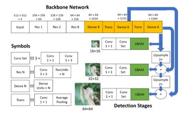
Figure 5: Proposed algorithm diagram

4. Experimental Setup

4.1.  Datasets

To evaluate the proposed method in this paper, two datasets, one for NLB and the other for gray leaf spot, are combined. For the first dataset, the Field images of maize annotated with disease symptoms dataset [25] was used. The dataset consists of natural environment 4000×6000 pixel images of maize leaves taken by hand during the 2015 growing period in Aurora, New York. The main axis of the NLB lesions in each image is annotated with line annotations. 376 images are extracted. Because of the high image resolutions, each image is split into a 2×3 grid for pixel preservation. For the original line annotations, multiple lines would be used to signify one contingent lesion when only one label should be used. As a result, annotations are reconverted into bounding box format by hand under the supervision of the original line annotations. Figure 6 shows the annotation process. Images without lesions are discarded, resulting in 999 final images. Data augmentation using random rotation and zoom was then used to 4x the dataset size.

Unlike for NLB, high quality datasets for gray leaf spot disease taken from the natural environment and annotated by experts are rare. Although an annotated gray leaf spot dataset from Plant Doc exists, as mentioned in the related works section, few images are provided. Additionally, clusters of spots are grouped as one label, as opposed to the individual disease symptom labeling that the format of the NLB dataset is in. As a result, the Plant Village dataset was chosen to be annotated, starting from scratch. Because the dataset was initially intended for CNN training, annotations are not provided. As a result, like the NLB dataset, new annotations around each spot were created. However, in the gray leaf spot dataset, no expert guidance was provided, meaning best guesses for what constituted a spot were made. Figure 7 shows examples of grey spot annotations. Although fewer images of gray leaf spot were used compared to NLB, more annotations per image for gray were created, balancing the total number of annotations per class. The Plant Village dataset, in addition to the gray leaf spot, contains healthy corn images. 200 healthy images from each dataset were added. Several dataset groupings were used in this study.

Table 1: Dataset description

Dataset	Training images	Validation images	Testing images	Total label count
NLB	3,145	135	135	5,255
Gray	608	24	30	5,677
NLB+Gray	3,753	159	165	10,932
Healthy	4,033	219	225	10,932

Dataset NLB: NLB infected images only, Dataset Gray: Gray leaf spot infected images only, Dataset NLB+Gray: only NLB and gray leaf spot images, and finally, Dataset Healthy: a combination of dataset NLB+Gray with healthy images. Healthy images from the original NLB and Plant Village datasets were also included so that the algorithms could better learn what is not considered diseased through more examples. More info regarding dataset size and label counts is shown in Table 1. Data is available at a project github site^a.

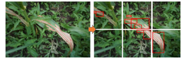
Figure 6: NLB annotation process

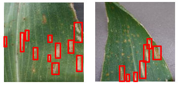
Figure 7: Grey leaf annotation examples

4.2.  Evaluation Metrics

Evaluating accuracy for object detection algorithms requires comparing both the label and location of the predicted bounding box to those of the ground truth. IoU, i.e., intersection over union, as given in equation (1), is the value of the intersection area of the bounding box, AreaPred, and the area of the ground truth box, AreaTruth, over the union area of the two aforementioned boxes.

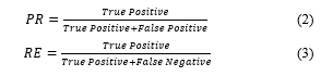
 If IoU is above a certain threshold value, that prediction is counted as a true positive. If not, it is considered a false positive. As shown in equation (2), precision, or PR, is the number of true positives divided by the sum of the number of true positives and false positives. Recall, or RE, shown in equation (3), is the number of true positives divided by the true positives and false negatives.

Average precision, i.e., AP, is calculated by finding the area under the precision-recall curve, shown in formula (4). P(r) is the precision value at recall value r. AP subscript k indicates the average precision when IoU is at threshold k.  indicates average precision at the 0.5 IoU threshold. If three lesions had IoU of 0.2, 0.6, and 0.3, only the lesion with the IoU 0.6 would be counted as a true positive.

Inference speed, parameter count, and MFLOPs were also measured. MFLOPs is a unit for how many million floating point operations per second the computer can operate. All results were tested on the same GPU and Google colab environment settings for fair comparisons.

5. Results

Model training and evaluation were done on colab with an Nvidia P100 GPU, Intel Xenon 2.2 GHz CPU, and 13 GB of RAM. Code implementations were done using TensorFlow 1.15.0 and Keras 2.1.6 with Python 3.7. The three different algorithms, (i) Base, (ii) Dense, and (iii) Dense-attention were trained and evaluated on images sized 512512 pixels.

Table 2 shows the  of the algorithms on the datasets On the NLB dataset, Base, Dense, and Dense-attention had  of 0.774, 0.806, and 0.821, respectively. In the Gray dataset, Base, Dense, and Dense-attention had of 0.484, 0.471, and 0.496, respectively, showing that locating the exact boundaries of the grey spot is much more complicated than finding NLB lesions. One of the possible reasons for this is that NLB may appear more distinctive in the images since the lesions in the images tend to appear brighter than lesions in the Gray dataset. In the NLB+Gray dataset, individual was recorded for each class. The for each class decreased slightly compared to detecting them in dataset NLB and dataset Gray, in which only one class was present in each, which is expected as multiclass detection is more difficult than single class detection. The slight decrease in  also indicates that the model has learned to differentiate NLB and Gray leaf spot. In the Healthy dataset, the usage of images of healthy images decreased performance. All results for healthy were worse than the results for the NLB+Gray dataset. Base outperformed Dense and Dense-Attention in terms of finding NLB lesions, with  of 0.714, 0.675, and 0.702, respectively. However, in terms of finding gray lesions, Dense-attention’s  of 0.473 was still higher than Base’s  of 0.425. One possible reason that adding healthy images did not help performance is that the healthy images may have simply included more objects that looked like lesions, such as a dry or dead leaf, which are common, making training harder for the models.

Table 2: Performance of algorithms measured in

Dataset	Base	Dense	Dense-attention
NLB	0.774	0.806	0.821
Gray	0.484	0.471	0.496
NLB lesions in NLB+Gray	0.769	0.763	0.785
Gray lesions in NLB+Gray	0.459	0.448	0.483
NLB lesions in Healthy	0.714	0.675	0.702
Gray lesions in Healthy	0.425	0.428	0.473

      Examples of detections are shown in Figure 8 and 9. Figure 8 shows detections of NLB by the Dense-attention trained from the NLB+Gray dataset. Figure 9 shows detections of Grey spot, also by Dense-attention trained from NLB+Gray. In Figure 9, it can be shown that the model has difficulty determining if two lesions close to each other are one or two lesions, as shown in the top row. In the bottom row, it can be shown that the model also has difficulty finding very small lesions.

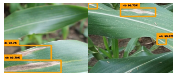
Figure 8: NLB detection of Dense-attention trained on NLB+Gray dataset

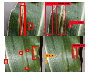
Figure 9: Gray detections of Dense-attention (right column) trained on NLB+Gray dataset side by side with ground truth (left column)

Table 3: General algorithm performance

Algorithm	Inference Speed (ms)	Parameters (millions)	MFLOPs
Base	36.9	61.5	123.0
Dense	37.4	40.8	81.6
Dense-attention	39.1	40.9	81.7

Table 3 shows the general performance of the algorithms, which shows constant results for the algorithms, no matter what dataset is used. Base has the fastest inference speed of 36.9 ms, followed by Dense with a speed of 37.4 ms, and finally Dense-attention, with a speed of 39.1 ms. There is not much of a major difference in inference speeds among all three algorithms. The usage of dense blocks to replace several layers of the original YOLOv3 backbone has greatly reduced the number of parameters. Base has 61.5 million parameters, Dense has 40.8 million, and Dense-attention has 40.9 million. The usage of CBAM has only increased the number of parameters slightly. The ratios of the parameter count between the algorithms are similar to the ratio of MFLOPs. Base has 123.0 MFLOPs, Dense 81.6, and Dense-attention 81.7. While Base is the fastest, Dense and Dense-attention are similar in speed while having drastically fewer parameters and MFLOPs. In terms of accuracy, Dense seems to have similar results with Base, although it was more accurate in the NLB dataset. Dense-attention, based on the results shown in Table 2, mostly outperforms both Base and Dense-attention.

6. Conclusion

The new proposed model, called dense-attention, was built off of YOLOv3 and optimized for both accuracy and speed. New datasets for NLB and gray leaf spot were created and reannotated to be more suitable for object detection tasks. The results showed that dense-attention outperformed the base model in terms of accuracy, parameter count, and computational efficiency, although it was slightly slower. When both NLB and gray leaf spot were combined in the dataset, performance for each class decreased slightly compared to training on just one of the diseases. This suggests that the model was able to distinguish between the two visually similar diseases. In future work, it may be helpful to annotate the gray leaf spot dataset with experts and to include wider views of diseased leaves in the dataset.

1. S. Savary, L. Willocquet, S. J. Pethybridge, P. Esker, N. McRoberts, A. Nelson, “The global burden of pathogens and pests on major food crops,” Nature Ecology & Evolution, 3(3), 430–439, 2019, doi:10.1038/s41559-018-0793-y.
2. T. M. Chaloner, S. J. Gurr, D. P. Bebber, “Plant pathogen infection risk tracks global crop yields under climate change,” Nature Climate Change, 11(8), 710–715, 2021, doi:10.1038/s41558-021-01104-8.
3. M. McConnell, “Feedgrains sector at a glance,” USDA Economic Research Service U.S. Department of Agriculture, 27 January 2023, https://www.ers.usda.gov/topics/crops/corn-and-other-feed-grains/feed-grains-sector-at-a-glance/.
4. D. S. Mueller et al., “Corn yield loss estimates due to diseases in the United States and Ontario, Canada from 2012 to 2015,” Plant Health Progress, 17(3), 211–222, 2016, doi:10.1094/PHP-RS-16-0030.
5. J. P. Zubrod et al., “Fungicides: An Overlooked Pesticide Class?”, Environmental Science & Technology, 53(7), 3347–3365, 2019, doi:10.1021/acs.est.8b04392.
6. K. Wise, “Northern corn leaf blight – purdue extension,” Purdue University, 2011, https://www.extension.purdue.edu/extmedia/BP/BP-84-W.pdf.
7. B. Song, J. Lee, “Detection of Northern Corn Leaf Blight Disease in Real Environment Using Optimized YOLOv3,” 2022 IEEE 12th Annual Computing and Communication Workshop and Conference (CCWC), 2022, 0475-0480, doi:10.1109/CCWC54503.2022.9720782.
8. S. P. Mohanty, D. P. Hughes, M. Salathé, “Using deep learning for image-based plant disease detection,” Frontiers in Plant Science, 7, 2016, doi:10.3389/fpls.2016.01419.
9. C. DeChant, T. Wiesner-Hanks, S. Chen, E. L. Stewart, J. Yosinski, M. A. Gore, R. J. Nelson, H. Lipson, “Automated identification of northern leaf blight-infected maize plants from field imagery using Deep Learning,” Phytopathology®, 107(11), 1426–1432, 2017, doi:10.1094/PHYTO-11-16-0417-R.
10. W. Liu, D. Anguelov, D. Erhan, C. Szegedy, S. Reed, C.-Y. Fu, A. C. Berg, “SSD: Single shot multibox detector,” Computer Vision– ECCV 2016, 21–37, 2016, doi:10.1007/978-3-319-46448-0_2.
11. P. Jiang, Y. Chen, B. Liu, D. He, C. Liang, “Real-Time Detection of Apple Leaf Diseases Using Deep Learning Approach Based on Improved Convolutional Neural Networks”, IEEE Access, vol 7, 59069–59080, 2019, doi:10.1109/ACCESS.2019.2914929.
12. J. Redmon, A. Farhadi, ‘YOLOv3: An Incremental Improvement’, arXiv, 2018, doi:10.48550/ARXIV.1804.02767.
13. J. Liu, X. Wang, “Tomato diseases and pests detection based on improved Yolo v3 convolutional neural network,” Frontiers in Plant Science, 11, 2020, doi:10.3389/fpls.2020.00898.
14. S. Ghoury, C. Sungur, A. Durdu, “Real-Time Diseases Detection of Grape and Grape Leaves using Faster R-CNN and SSD MobileNet Architectures,” International Conference on Advanced Technologies, Computer Engineering and Science (ICATCES 2019), 39-44, 2019 Alanya, Turkey.
15. S. Ren, K. He, R. Girshick, J. Sun, “Faster R-CNN: Towards real-time object detection with region proposal networks,” IEEE Transactions on Pattern Analysis and Machine Intelligence, 39(6), 1137–1149, 2017, doi:10.1109/TPAMI.2016.2577031.
16. M. H. Saleem, S. Khanchi, J. Potgieter, K. M. Arif, “Image-Based Plant Disease Identification by Deep Learning Meta-Architectures,” Plants, 9(11), 1451, 2020, doi: 10.3390/plants9111451.
17. D. Singh, N. Jain, P. Jain, P. Kayal, S. Kumawat, N. Batra, “Plantdoc,” Proceedings of the 7th ACM IKDD CoDS and 25th COMAD, 2020, doi:10.1145/3371158.3371196.
18. J. Redmon, S. Divvala, R. Girshick, A. Farhadi, ‘You Only Look Once: Unified, Real-Time Object Detection’, Proceedings of the IEEE Conference on Computer Vision and Pattern Recognition (CVPR), 2016, doi:10.1109/CVPR.2016.91.
19. J. Redmon, A. Farhadi, ‘YOLO9000: Better, Faster, Stronger’, Proceedings of the IEEE Conference on Computer Vision and Pattern Recognition (CVPR), 6517-6525, 2017, doi:10.1109/CVPR.2017.690.
20. A. Bochkovskiy, C.-Y. Wang, H.-Y. M. Liao, ‘YOLOv4: Optimal Speed and Accuracy of Object Detection’, arXiv, 2020, doi:10.48550/ARXIV.2004.10934.
21. K. He, X. Zhang, S. Ren, J. Sun, ‘Deep Residual Learning for Image Recognition’, Proceedings of the IEEE Conference on Computer Vision and Pattern Recognition (CVPR), 770-778, 2016, doi: 10.1109/CVPR.2016.90.
22. C.-Y. Fu, W. Liu, A. Ranga, A. Tyagi, A. C. Berg, ‘DSSD : Deconvolutional Single Shot Detector’, arXiv, 2017, doi: 10.48550/ARXIV.1701.06659
23. G. Huang, Z. Liu, L. Van Der Maaten, K. Q. Weinberger, ‘Densely Connected Convolutional Networks’, 2017 IEEE Conference on Computer Vision and Pattern Recognition (CVPR), 2261–2269, 2017, doi:10.1109/CVPR.2017.243.
24. S. Woo, J. Park, J.-Y. Lee, I. S. Kweon, ‘CBAM: Convolutional Block Attention Module’, Proceedings of the European Conference on Computer Vision (ECCV), 11211, 3-19, 2018, doi: 10.1007/978-3-030-01234-2_1.
25. T. Wiesner-Hanks, E. L. Stewart, N. Kaczmar, C. DeChant, H. Wu, R. J. Nelson, H. Lipson, M. A. Gore, “Image set for Deep Learning: Field images of maize annotated with disease symptoms,” BMC Research Notes, 11(1), 2018, doi:10.1186/s13104-018-3548-6.

(Click Here)