1. Introduction

Sleep acts as a vital part of the physical health and quality of human lives. Sleep diseases, like obstructive sleep apnea (OSA) and insomnia, might result in daylight drowsiness, depression, or even mortality [1]. Thus, there is a need to design an efficient method for diagnosing and treating sleep-related diseases. The study of sleep-related diseases is labeled “sleep medicine,” which was once a significant medical field and has been included in various medical challenges. It consists of two major categories of sleep namely, rapid eye movement (REM) sleep and nonrapid eye movement (NREM). The REM and NREM sleep stages are adjacent and alternated by the sleep procedure on a regular basis, and unbalanced cycling or the absence of a sleep stage results in a sleep disorder [2]. Inappropriate sleep disorders result in inferior quality of sleep, which is frequently ignored and emphasized that sleep-related issues are a forthcoming worldwide health problem [3]. Sleep stage classification is the initial phase of the diagnosis of sleep-related diseases[4] . The critical stage in sleep research is collecting the polysomnographic (PSG) information from the patient at the time of sleep. The PSG information comprises electromyography (EMG), electroencephalography (EEG), bio-physiological signal, electrocardiography (ECG), and respiratory efforts. Until recently, the sleep stage score had to be physically determined by human experts [5].

A human expert’s ability to manage slower changes in background EEG is limited, and he or she learns the distinct guidelines for scoring sleep stages from multiple PSG recordings [6]. Moreover, the calculations by the sleep expert are inclined to inter and intra- observer variability, which influences the quality of the sleep stage score. This substantiates the need for sleep stage scoring using Artificial Intelligence (AI) techniques[7].

Sleep stage classification has been studied for several years, and different advanced techniques and medical application areas have been established. ML techniques used for SSC are artificial neural networks (ANN), support vector machines (SVM), dual-tree, K-means clustering, and empirical mode decomposition (EMD). However, these traditional methods rely on the detection of biological signals [8]. The manual features are created from the EEG signal, which has a tendency toward local optimization. Moreover, the patterns of brain signals are complex compared to the present knowledge of human beings, which might result in data loss in the manual way of extracting features. Additionally, feature extraction is a difficult and lengthy process. It also necessitates excessively long working hours for experienced experts. The convenience and accuracy of sleep stage classification techniques are critical issues in the analysis of sleep-related diseases.

In recent times, different studies have utilised deep learning (DL) models, which are motivated by the biological imitation outcomes of the visual cortex of mammals. In contrast to the conventional technique, it decreases the difficulty of the network and weight count due to its shared weight networking model, which is equivalent to a biological NN. Additionally, it reduces the calculation process because of its capability of classifying the EEG data without hand-crafted feature extraction.

This paper presents DL models with AR regularisation functions and ensemble DL models for sleep stage classification. At the initial stage, the required features were extracted from the single channel and normalized. Following this, the proposed model employed three DL models, namely, the recurrent neural network (RNN), long short-term memory (LSTM), and gated recurrent units (GRU), for classifying the sleep stages. At last, the presented model integrates the results of every classification model using the max voting combination rule to generate an optimal outcome. The experimental analysis was performed to highlight the improvements of the proposed model over the existing models.

The construct of the paper is detailed as follows: Section 2 summarizes an overview of the existing work based on deep learning techniques for sleep stage classification. Section 3 provides an overview of the proposed work for SSC using DL models, various Regularization, and ensemble techniques. Section 4 discusses the dataset details, implementation details, and performance evaluation of the proposed work. Section 5 provides conclusion on performance on proposed model on sleep stage dataset.

2. Related works

The author proposed an NN-based CNN with an attention scheme for automated sleep stage classification. The weighted loss function employed in the CNN model handled the class imbalance problem for sleep stage classification [9].  Developed an automated DL-based sleep stage classification model utilizing EEG signals that automatically extracted the time-frequency spectra of the EEG signals. The Continuous Wavelet Transform (CWT) technique was used for extracting the RGB color images of the EEG signal. The transfer learning of the pre-trained CNN was utilised to classify the CWT images according to sleep levels [10].

Developed an orthogonal convolutional neural network (OCNN) for learning rich and efficient feature representation. The Hilbert-Huang transform was used to extract the time-frequency representation of the EEG signal, and OCNN was used to classify the sleep stages [11]. An effective ensemble method to classify distinct types of sleep stages. The classification technique was employed an integration of the EEGNet and BiLSTM models for learning the distinct features of EEG and EOG signals, respectively [12].

In the past few decades, the sleep stage classification process has gained significant attention. Machine learning techniques such as multiclass SVM, and linear discriminant analysis were applied for classifying sleep stages [13]. Proposed a technique for detecting sleep stages based on iteration filtering. The amplitude envelope and instantaneous frequency (AM-FM) were applied for classifying the sleep stages, and an average accuracy of 86.2% across five sleep stages was achieved[14] .

The author proposed a novel sleep stage recognition method based on a new set of wavelet-based features extracted from massive EEG datasets. The integrated SVM technique and CNN model were employed on the EEG signal for extracting features and classifying the sleep stages. It was implemented to learn task-oriented filters to classify data depending on single-channel EEG without utilizing previous domain information [15].

The author proposed a deep CNN framework extracted data from raw EGG signals and classified the sleep stages using the SoftMax activation function[16]. Smart technology for sleep stage classification was developed, data were trained using two different fuzzy rule algorithms for classifying sleep stages and studying the new patient’s record. But it ignores the connection between the current stage and its adjacent sleep stage and does not capture the transition rules among the sleep stages [17].

An Elman RNN was proposed for automatically classify sleep staging systems. This system classified different sleep stages based on energy features (E) of 30 s epochs extracted from a single channel’s EEG signals [18]. The author proposed DeepSleepNet model extracted time-invariant features from the EEG signal using CNN and bi-directional LSTM and learned the stage transitions rule. Also, the two-step training algorithm was used to lessen class-imbalance problems and encode the temporal information of the EEG signal into the model [19]. The author developed a mixed neural network (MLP and LSTM), the temporal physiological features of the signal were extracted using power spectral density (PSD), and the extracted features were classified using an MLP and LSTM [20]. The sequential feature learning model was developed using a deep bi-directional RNN with an attention method for single-channel automated sleep stage classification. The time-frequency features were extracted from the EEG [21].

The sleep stage classifier technique was proposed, the temporal (59) and frequency domain (51) characteristics of the EEG signal were extracted using the PSD approach, and the extracted features were classified using the C-CNN and attention-based BiLSTM models [22]. The author proposed SleepEEGNet combines the CNN and BiLSTM models to extract the time and frequency features and capture the sleep transition between the epochs in a single-channel EEG signal. The new loss function technique in the SleepEEGNet decreases the effects of the class imbalance problems [23].

The author developed a classification framework for automatic sleep stage recognition from a combination of male and female human subjects. Then the ResNet structure automatically extracts the frequency features from the raw EEG signal [24].

Transfer learning-CNN was developed for classifying the sleep stages. The time and frequency features were calculated using PSD estimation and statistical techniques from the EEG and EOG signals. The EEG feature set and the set of fused features of EEG and EOG signals were separated and converted into image sets using a horizontal visibility graph (HVG) in Euclidean space. An image of HVG is classified into different sleep stages using transfer learning-CNN [25].

3. Proposed Sleep Stage Classification Model

The workflow involved in the proposed model for SSC is given in Figure. 1. The figure shows that the initial stages of the processing of input EEG data involve data extraction of sub-band frequency and data normalization. Followed by three DL models with activity regularization techniques are used for the classification of EEG signals for SSC. Finally, the max voting ensemble method is applied to determine the performance of the optimal sleep state classification results of the presented model.

3.1.  Data acquisition and Preprocessing

The multichannel time series data is extracted from different channels of EEG (Fpz-Cz), Pz-Oz, and EOG. The EEG signal is recorded by positioning the electrode in accordance with the International 10-20 systems. The EEG data from a single EEG channel (Fpz-Cz) is considered for this research work. The steps for extracting the EEG signal data that is fed into the DL model are narrated as follows:

• The extracted EEG signal (time series) of 30-sec epochs is fed as input to the DL models.
• The continuous raw signal is converted into sequential data of 30 s epochs is segmented, and stages of S1, S2, S3/4, wake, and REM are assigned in each epoch based on the annotation file in the AASM standard.
• Since each segment(fragment) of 30 s epochs was sampled at 100Hz, and 3000- time points (30*100) for five stages, are extracted.

The power spectral density (PSD) technique is applied to extract different sub-bands frequencies (35 features) from the EEG signal to identify each stages correctly. The signal is then normalized to have a zero mean and unit variance for each of the 30-second epochs and divided by each segment’s power spectral density of each frequency band (0.5 to 30 Hz) by each segment’s total power spectral density. The power spectral intensity of the kth is measured by Eq. (1).

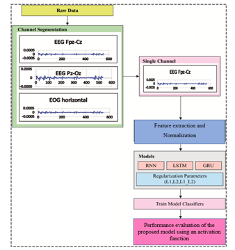
Figure 1: Overall Process of Proposed DL model

3.2.  DL Models

The DL models LSTM, GRU, and RNN are discussed in the following section.

3.2.1. RNN Model

RNN is a kind of NNs with loops that permits persisting data from the past in the neural network system. In Figure. 2, the center square signifies a NN that takes input  at present time step  and provides the value  as an outcome. The loop in the model allow to utilize data from the previous time step for producing output at the present time like step . So, it is the state that the decision develops at time slice  influences the decisions to be developed at time step . Thus, the RNN output for the novel information is based on the present input and recent past output data [26]. The RNN output computation depends on the frequent computation of the outcome using Eqn. (2)-(3):

where  implies the input order at the current time step    represents the output order at time step , and  signifies the order of the hidden vectors in the time step 1 to T.  and  denotes weight matrix as well as bias correspondingly.

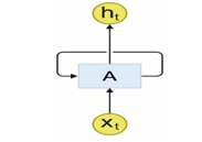
Figure 2: Loop structure of RNN

3.2.2. LSTM Model

Hochreiter and Schmidhuber introduced the LSTM networks in 1997 [27].LSTM is a different kind of RNN with memory cells. These memory cells are important to manage long-term dependencies on the information. The chain like architecture of LSTM is as shown in Figure 3 and specific memory cells from LSTM. All large square blocks imply the memory cell. The cell states are an important portion of the LSTM model which are represented through the horizontal line moving with the top of cell from the Figure. It executes in all cells from the chain of LSTM networks. The LSTM takes the possibility of adding or deleting data in the cell state. This function is completed by other architecture in LSTM known as gates. The gates are computed using the sigmoid  activation function (demonstrated by  in Figure. 3) and point-wise multiplication function (illustrated  in Figure. 3). They are 3 gates that manage data to pass with the cell state. The forget gate is responsible to remove information from the cell state. Besides, the input gate is accountable for appending information to the cell state. The output gate elects the data of the cell state to the outcome.

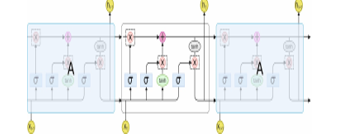
Figure 3: Architecture of LSTM model

The computation in the typical single LSTM cell can be expressed by:

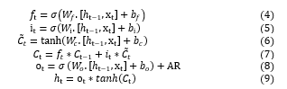
where the activation function utilized is sigmoid function  and hyperbolic tangent function ,       signifies the input gate, forget gate, output gate respectively,     memory cell current content, new cell state, hidden state correspondingly. Every W and b refer to the weight matrix and bias, respectively.

3.2.2. GRU Model

The GRUs are the other kind of RNNs with memory cells. The GRU also takes a gating scheme for controlling the flow of data with cell state but takes few parameters and does not comprise an output gate. The GRU has 2 gates,  implies the reset gate, and  represents the update gate is as shown in Figure 4. The reset  gate controls the new input data and decides how much of the past information should be forgotten. The update gate updates the information of the previous state and carries that information (data) for a prolonged period [28].

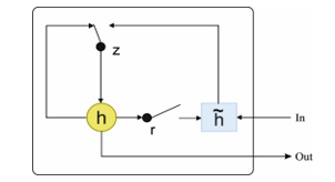
Figure 4: Structure of GRU model

The subsequent formulas are utilized in GRU outcome computations:

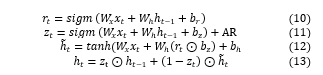
In Eqs. (10)-(13),        implies the input vector, output vector, reset gate, and an updated gate correspondingly. Every  variable refers to the weight matrix, and  signifies the bias. The following section discusses various regularization techniques.

3.3.  Regularization Functions

Overfitting is a prominent issue in the deep learning model, which prevents from completely generalizing the models to fit perfectly on the validation set during training. During the initial stage of training, the validation error decreases typically along with the error on the training set. However, the validation set error will increase as the model starts to overfit the data. Overfitting in the learning curve while training the model is as shown in Figure 5. The learning curve is a graphical plot of learning the data and diagnosing the model’s learning performance through loss values (y-axis) with respect to epochs (x-axis). The performance of the deep learning model creates a vast gap, resulting in random fluctuations between the training loss (high performance) and the validation loss (lower performance) while training and evaluating the model.

The overfitting of data happens because of the following reasons.

The model comprises of more than one hidden layer stacked together with nonlinear information processing to learn the association between input and output data and the learning of the association is a complex process.

• Additionally, deep neural networks’ loss function/cost function is highly nonlinear and not convex [29].

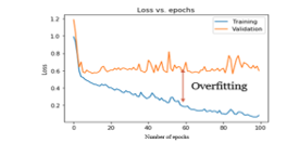
Figure 5: Overfitting (Learning curve)

3.3.1. Purpose of regularization

In the literature, to overcome the overfitting problem, various regularization techniques are adopted. The “activity regularization” technique is applied to the DL models to improve the performance to a great extent, mainly when an overfitting problem occurs [30]. It can be applied either to the hidden layers or the output layers of the DL models. It aids minor changes in the weight matrix of the learning approach while learning the data and thus reduces generalisation errors.

3.4. Various Regularization techniques

In this section various activation regularization techniques are discussed below.

L1 activation (Activity) regularization (AR): The L1(AR) technique is applied to the activation function in the DL model. L1 Regularization is calculated as the “sum of the absolute activation values.” The L1 AR causes the activation values to be sparse, thus allowing specific activations to reach zero. The L1 norm may be a more commonly utilised activation Regularization penalty [31].

L2 activation (Activity) regularization: L2 (AR) Regularization is calculated as the “sum of the squared activation values.” L2 Regularization keeps the magnitude of activations small, allowing specific activation values other than zero [32].

In this research work, L1, L2, and L1_L2 Regularization techniques alone are used for the experiments, which aid in better decision-making and prediction. This technique aids in improving the learning process in the DL models, thereby reducing generalisation errors.

3.4. Ensemble techniques

The ensemble technique combines the decisions/predictions from multiple models to make a final prediction and is used to enhance the model’s performance. The simple ensemble techniques of majority voting is as shown in Figure 6.

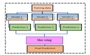
Figure.6: Simple Ensemble Techniques

Majority (max) ensemble voting

In max voting technique, the output of the multiple DL models is combined using the max-voting technique to make final predictions/decisions. The model classifies the instance to 1 and 0 otherwise for the  class of the  model [33].

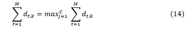
where  , M- is the number of model classifiers and k=1,2……., C, C -is the number of classes.

4. Implementation

4.1. Dataset Details

The sleep staging datasets from the physionet consist of 197 recordings of PSG signals, including 153 sleep cassettes (SC) of healthy patients and 44 sleep telemetry (ST) patients with medication. The details associated with the sleep dataset for 15 subjects are as given in Table 1. The sleep dataset contains bipolar channels (Fpz-Cz and Pz-Oz). The single channel (Fpz-Cz) indicates that the brain activity related to sleep stage connectivity is located in the cerebral midline. The DL model quickly learns the sequential features from a single channel (Fpz-Cz) to minimize the processor’s load and computational time. The channel selection process involves choosing a single channel for the sleep stage classification process. This work using three DL models to automatically classify sleep stages using a single channel (Fpz-Cz) from EEG signals (physionet.org).

Table 1. Dataset Details

Dataset	Wake (W)	S1 (N1)	S2 (N2)	S4 (N3-N4)	REM	Total Epochs
Sleep-EDF-18	8006	635	3621	1299	1609	15,170

In this dataset, 10% of patients do not have alpha waves during w. Sleep stage scoring is a time series (sequential) problem, so it depends on temporal features and previous epochs of the sleep stages (the N2 stage depends on the N1). The benchmark sleep stage dataset (physionet) was used in the experiment to assess the performance of the DL models. This research work used recordings of data from fifteen (15) subjects, ages 25 to 101. The original recording consists of sleep stages labeled as W (wake), 1, 2, 3, 4, M (movement time), R (REM), and unknown (?). For experimental purposes, only five stages, viz., wake, REM, 1, 2, 3, and 4, are considered. In addition, movement time and unknown stages are not taken into consideration. Stages 3 and 4 are considered a single stage according to AASM standards. The DL model’s performance is measured using accuracy, recall, F-score, precision, and kappa coefficient.

4.2. Platform used for Implementation.

Keras is one of the deep learning libraries that supports the implementation of complicated pre-packaged architectures like RNN, GRU, and LSTM. The DL model experiments were conducted on an Intel Core i5 processor with 16 GB of RAM. The deep learning models were developed using the Python programming language. The training parameters for the SSC dataset are tabulated in Table 2. The parameters of each DL model were fixed by conducting several experiments and considering various combinations; the model that produced the best results was saved for this research work.

Table 2. Experimental design and Training parameters

Parameter	Value
Batch size, Epochs, and optimizer	32, 100 and SGD respectively
Layer one	Sequential input layer
Layer 2 RNN/LSTM /GRU	90 (Number of neurons)
Layer 3 RNN/LSTM /GRU	50 (Number of neurons)
Layer 4 Fully connected layer	10 (Number of neurons)
Layer 5 Output layer	5 SoftMax AF

 5. Performance Evaluation

5.1. Experiments using RNN with (or) without regularization (WR)

The comparative result analysis of RNN model is evaluated with and without regularization as depicted in Table 3. The performance of the model is computed in terms of precision-recall, f-measure, training loss, validation loss, validation accuracy and training accuracy is given in Table 7. From the graph shown in Table 3, the performance of RNN-WR (without regularization) shows that there is a high gap and random fluctuation between validation loss and training loss, which indicates the onset of overfitting, as shown in Tables 3 (a) and 7.

Table 3. RNN learning curve with and without regularization

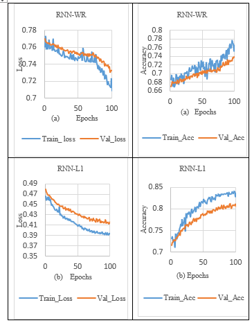
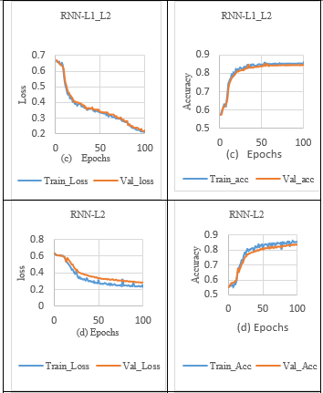
In order to overcome the overfitting problem in the RNN model, the L1 norm activity regularisation technique with a penalty value of 0.001 was applied to the RNN layer. It is observed that validation loss is reduced but fails to close the gap between the training loss and validation loss in the sleep stage classification process, as shown in Tables 3 (b) and 7. In addition, when the L1_L2 norm activity regularization technique with a penalty value of 0.001 was set to the RNN layer, the significant gap between the training and validation loss were minimised, which increased the validation accuracy, as shown in Table 3. (c) and 7.

Besides, the L2 norm activity regularization technique with a penalty value of 0.001 to the RNN layer, reducing validation loss, and slightly closing the gap between the training loss and validation loss. So, the RNN model with L2 regularization achieved lower validation loss and higher validation accuracy, as shown in Table 3. (d) and 7. The RNN models with and without the regularization effect were integrated using the max voting technique to make the final prediction of ensemble models. At last, ensemble RNN achieved lower validation and training loss indicates no sign of overfitting as shown in Table 3 (e). Also, the ensemble model exhibit on-par performance with the effect of adding combined regularization (L1_L2) for sleep stage classification in the RNN model, as shown in Table 3. (c) and 7.

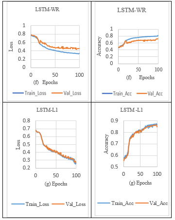
5.2.  Experiments using LSTM with (or) without regularization

Table 4 shows the LSTM model’s comparative result analysis. The LSTM model results are evaluated using metrics such as training loss, validation accuracy, validation loss and training accuracy, which are also computed and reported. As shown in Tables 4 (f) and 7, the performance of LSTM-WR (without regularization) for sleep stage classification during training predicts the output with a lower training loss and a higher validation loss, indicating the sign of overfitting. Overcome the overfitting problem in the LSTM model, the L1 norm activity Regularization technique with a penalty value of 0.001 was applied to the LSTM layer. It is observed from Table 7 that LSTM with L1 Regularization achieved a loss difference of 0.0231, which indicates validation loss is reduced and slightly closes the gap between the training and validation losses in the sleep stage classification, as shown in Tables 4 (g) and 7.

Table 4. LSTM learning curve with and without regularization

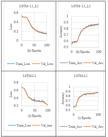
In addition, the L1_L2 norm activity Regularization technique with a penalty value of 0.001 was applied to the LSTM layer. It is observed in Table 7. that LSTM with L1_L2 activity Regularization achieved a loss difference of 0.0111, which effectively closed the significant gap between the training and validation losses, thus increasing validation accuracy, as shown in Tables 4(h) and 7.

Besides, the L2 norm activity Regularization technique with a penalty value of 0.001 was applied to the LSTM layer. It is observed from Table 7 that LSTM with L1 Regularization achieved a loss difference of 0.012, reducing validation loss and closing the gap between the training loss and validation loss. So, the LSTM model with L2 regularization achieved lower validation loss and higher validation accuracy, as shown in Tables 4 (i) and 7.

The LSTM models with and without the Regularization effect are combined using the max voting technique to make the final prediction of ensemble models. At last, ensemble LSTM attained higher performance with lower validation and training losses, which achieved a loss difference of 0.0013, indicating no sign of overfitting, as shown in Tables 4 (j) and 7. To conclude, the ensemble LSTM model exhibits higher performance and closes the gap between training loss and validation loss for SSC.

5.3.  Experiments using GRU with (or) without regularization

Table 5 depicts the GRU model’s comparative result analysis. From the graph shown in Table 5, the performance of GRU-WR (without Regularization) for the sleep stage classification model attained a lower training loss and a higher validation loss, which discloses the sign of overfitting, as shown in Tables 5 (k) and 7. Overcome the overfitting problem in the GRU model, the L1 norm activity Regularization technique with a penalty value of 0.001 was applied to the GRU layer.

It is observed from Table 7 that GRU with L1 Regularization achieved a loss difference of 0.0231, which indicates validation loss is reduced but failed to close the gap between training and validation loss in the sleep stage classification process, as shown in Tables 5 (l) and 7.

In addition, the L1_L2 norm activity regularization technique with a penalty value of 0.001 was applied to the GRU layer. It is observed from Table 7 that GRU with L1_L2 Regularization achieved a loss difference of 0.0018, which effectively closed the significant gap between the training and validation loss, thus increasing validation accuracy, as shown in Tables 5 (m) and 7.

Table 5. GRU learning curve with and without Regularization

 

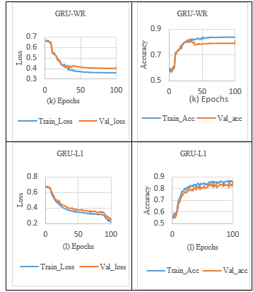
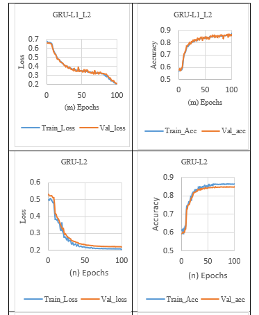
Besides, the L2 norm activity Regularization technique with a penalty value of 0.001 was applied to the GRU layer. It is observed from Table 7 that GRU with L1 Regularization achieved a loss difference of 0.0158, reduced validation loss, and slightly closed the gap between the training loss and validation loss. So, the GRU model with L2 Regularization achieved lower validation loss and higher validation accuracy, as shown in Tables 5. (n) and 7.

The GRU models with and without the regularization effect are combined using the max voting technique to make the final prediction of ensemble models. At last, ensemble GRU attained higher performance with lower validation and training loss, which achieved a loss difference of 0.0052, indicating no sign of overfitting, as shown in Tables 5 (o) and 7.

Table 7. Result analysis of DL models on sleep stage dataset

Models	Precision (%)	Recall (%)	F-Measure (%)	Training Loss	Training Accuracy (%)	Validation Loss	Validation Accuracy (%)
RNN-WR	74.33	76.67	75.48	0.7090	76.62	0.7329	73.71
RNN-L1	83.12	84.52	83.81	0.3310	83.62	0.4730	80.92
RNN-L1L2	85.41	89.21	87.27	0.2112	86.10	0.2264	85.03
RNN-L2	87.01	87.13	87.06	0.2242	85.78	0.2831	83.90
Ensemble RNN	85.82	89.84	87.78	0.2093	86.88	0.2221	85.57
GRU-WR	82.71	86.42	84.52	0.3115	84.42	0.4123	81.27
GRU-L1	88.09	89.36	88.72	0.2205	86.10	0.2436	84.14
GRU-L1L2	87.84	90.09	88.95	0.2060	87.90	0.2078	86.95
GRU-L2	87.94	89.48	88.7	0.2023	86.45	0.2181	85.25
Ensemble GRU	88.45	89.88	89.16	0.1977	88.08	0.2029	87.41
LSTM-WR	85.48	87.10	86.28	0.3533	85.45	0.5682	81.97
LSTM-L1	87.98	88.78	88.38	0.2551	86.56	0.2782	84.55
LSTM-L1L2	88.10	89.07	89.38	0.1420	88.75	0.1531	87.98
LSTM-L2	89.12	87.34	88.22	0.2225	87.21	0.2345	86.17
Ensemble LSTM (E-LSTM	88.98	90.76	89.86	0.1201	89.18	0.1214	89.01

Table 7 indicates the sleeping stage classification outcome of the different DL models with ensemble techniques. Figures. 7 illustrates the result analysis of different DL models with ensemble techniques on the sleep stage dataset.

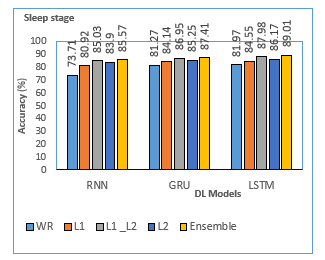
Figure. 7: Accuracy analysis of DL models for sleep stage

The ensemble models such as Ensemble RNN, Ensemble GRU, and Ensemble LSTM models have accomplished maximum validation accuracy of 85.57%, 87.41%, and 89.01%, respectively. Among the three DL models, the Ensemble-LSTM has established outstanding results and is considered a suitable model for sleep stage classification concerning good f-measure, higher accuracy of 89.01%, and lower validation loss.

Table 6. Per-class performance achieved by E- LSTM Models on SSC Dataset

Sleep stage	Predicted on SSC dataset					Evaluation metrics (%)
	W1	N1	N2	N3	REM	Precision	Recall	F-measure
W1	7726	206	42	32	21	96.25	96.58	96.19
N1	94	350	78	5	87	56.29	45.51	50.57
N2	90	104	3286	81	60	90.26	82.70	86.77
N3	76	24	140	1019	40	78.44	88.87	85.13
REM	60	146	163	32	1208	75.07	88.71	85.02
Overall		Accuracy=89.01 %				Kappa=0.838

Table 6. shows the per-class performance achieved by the ensemble LSTM model for the sleep stage dataset (single channel). The diagonal values in the confusion matrix represent True Positive (TP) and imply that the number of sleep stages is correctly classified. The table shows the classification performance of each stage in terms of precision, recall, overall accuracy, kappa, and f-score. The model performs better for stages W, N2, N3, and REM, except for N1. It may be because the N1 stages have fewer epochs than the other stages. However, ensemble LSTM achieved better performance when compared with other state-of-the-art models (cascaded, Elman, attentional RNN) except for the N1 stage, as shown in Table 8. The reason is that other models classified sleep stages using fewer sleep stage epochs. The kappa (k) values showed a significant level of agreement between the E-LSTM model and the sleep expert.

Table. 8. Comparative Accuracy analysis of the proposed E-LSTM with existing models

Models	Overall Metrics			Per-class F-Score
	Sleep stage total (Epochs)	Accuracy (%)	kappa	W	S1	S2	S3	REM
Attentional RNN	–	79.1	0.762	75.5	27.3	86.6	85.60	74.8
Elman	2880	87.20	–	70.8	36.7	97.3	89.70	89.5
Cascaded	10280	86.74	0.79	95.29	61.09	85.48	84.80	83.74
Proposed E-LSTM	15170	89.01	0.838	96.19	50.57	86.77	85.13	85.02

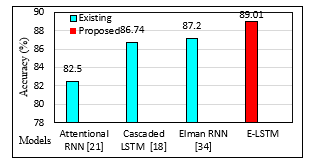
Figure. 8: Accuracy Analysis of the proposed E-LSTM with existing models

Table 8 shows a brief comparison of the ensemble models’ results with those of existing models. In terms of accuracy, Figure 8 compares the proposed E-LSTM model to existing models.

Using the SleepEDF -18 dataset, the attentional RNN model, cascaded, and Elman RNN were used in the literature for SSC. The proposed ensemble LSTM model’s performance is compared with that of the existing model, and the results are reported in Table 8. The results show that the attention mechanism has accomplished a lower accuracy of 79.10%. Cascaded and Elman RNN models have obtained moderate accuracy of 86.74% and 87.20% [34], respectively.

As previously mentioned, it is evident that the Ensemble LSTM model outperforms the other model on the SSC. The experimental result reported that the ensemble LSTM had attained a higher classification accuracy with a good F-score. Hence, the performance of the E-LSTM model for SSC is observed to be a better model than other models reported in the literature.

6. Conclusion

This paper has effectively designed an ensemble of voting-based DL models with Regularization functions for sleep stage classification. At the initial stage, the input EEG data is pre-processed in stages such as channel extraction, feature extraction, and data normalization. Subsequently, three DL models, namely the RNN, LSTM, and GRU models, are employed for the classification of EEG sleep stages. A comprehensive set of simulations was done to validate the effective sleep stage classification outcome of the presented model, highlighting the superior outcome of the presented model. The obtained experimental results highlighted the improvement of the presented model on the test EEG sleep state dataset. While training the applied DL models, activity Regularization techniques are used to mitigate the overfitting problem. The proposed model overcame the overfitting problem that affected the model’s performance. The DL model with activation Regularization techniques was used to close the gap between validation and training loss, which improved the model’s performance. The max voting technique is used to determine the optimal SSC efficiency of the presented model. The experimental results showed that the ensemble RNN, ensemble GRU, and ensemble LSTM models had achieved an accuracy of 85.57%, 87.41%, and 89.01%, respectively, for sleep stage classification. In the future, bio-inspired optimization algorithms can be employed to determine the optimal weights in the voting technique. Additionally, the sleep stage is a sequential time series of various sleep stages (sub-bands), so one stage depends on the previous stage.

Conflict of Interest

The authors declare no conflict of interest.

1. A.D. Laposky, J. Bass, A. Kohsaka, F.W. Turek, Sleep and circadian rhythms: Key components in the regulation of energy metabolism, FEBS Letters, 582(1), 142–151, 2008, doi:10.1016/j.febslet.2007.06.079.
2. J.C. Carter, J.E. Wrede, Overview of sleep and sleep disorders in infancy and childhood, Pediatric Annals, 46(4), e133–e138, 2017, doi:10.3928/19382359-20170316-02.
3. S. Stranges, W. Tigbe, F.X. Gómez-Olivé, M. Thorogood, N.B. Kandala, “Sleep problems: An emerging global epidemic? Findings from the INDEPTH WHO-SAGE study among more than 40,000 older adults from 8 countries across Africa and Asia,” Sleep, 35(8), 1173–1181, 2012, doi:10.5665/sleep.2012.
4. F. Mendonça, S.S. Mostafa, F. Morgado-Dias, J.L. Navarro-Mesa, G. Juliá-Serdá, A.G. Ravelo-García, “A portable wireless device based on oximetry for sleep apnea detection,” Computing, 100(11), 1203–1219, 2018, doi:10.1007/s00607-018-0624-7.
5. Z. Roshan Zamir, N. Sukhorukova, H. Amiel, A. Ugon, C. Philippe, Optimization-based features extraction for K-complex detection, 2013.
6. L. Wei, Y. Lin, J. Wang, Y. Ma, “Time-frequency convolutional neural network for automatic sleep stage classification based on single-channel EEG,” in Proceedings – International Conference on Tools with Artificial Intelligence, ICTAI, IEEE Computer Society: 88–95, 2018, doi:10.1109/ICTAI.2017.00025.
7. D. Wang, D. Ren, K. Li, Y. Feng, D. Ma, X. Yan, G. Wang, “Epileptic seizure detection in long-term EEG recordings by using wavelet-based directed transfer function,” IEEE Transactions on Biomedical Engineering, 65(11), 2591–2599, 2018, doi:10.1109/TBME.2018.2809798.
8. A. Ramachandran, A. Karuppiah, A survey on recent advances in machine learning based sleep apnea detection systems, Healthcare (Switzerland), 9(7), 2021, doi:10.3390/healthcare9070914.
9. T. Zhu, W. Luo, F. Yu, “Convolution-and attention-based neural network for automated sleep stage classification,” International Journal of Environmental Research and Public Health, 17(11), 1–13, 2020, doi:10.3390/ijerph17114152.
10. P. Jadhav, G. Rajguru, D. Datta, S. Mukhopadhyay, “Automatic sleep stage classification using time–frequency images of CWT and transfer learning using convolution neural network,” Biocybernetics and Biomedical Engineering, 40(1), 494–504, 2020, doi:10.1016/j.bbe.2020.01.010.
11. J. Zhang, R. Yao, W. Ge, J. Gao, “Orthogonal convolutional neural networks for automatic sleep stage classification based on single-channel EEG,” Computer Methods and Programs in Biomedicine, 183, 2020, doi:10.1016/j.cmpb.2019.105089.
12. I.N. Wang, C.H. Lee, H.J. Kim, H. Kim, D.J. Kim, “An Ensemble Deep Learning Approach for Sleep Stage Classification via Single-channel EEG and EOG,” in International Conference on ICT Convergence, IEEE Computer Society: 394–398, 2020, doi:10.1109/ICTC49870.2020.9289335.
13. R. Boostani, F. Karimzadeh, M. Torabi-Nami, A Comparative Review on Sleep Stage Classification Methods in Patients and healthy Individuals A Comparative Review on Sleep Stage Classification Methods in Patients and healthy Individuals A Comparative Review on Sleep Stage Classification Methods in Patients and healthy Individuals.
14. R. Sharma, R.B. Pachori, A. Upadhyay, “Automatic sleep stages classification based on iterative filtering of electroencephalogram signals,” Neural Computing and Applications, 28(10), 2959–2978, 2017, doi:10.1007/s00521-017-2919-6.
15. M. Sharma, D. Goyal, P. v. Achuth, U.R. Acharya, “An accurate sleep stages classification system using a new class of optimally time-frequency localized three-band wavelet filter bank,” Computers in Biology and Medicine, 98, 58–75, 2018, doi:10.1016/j.compbiomed.2018.04.025.
16. S. Chambon, M. Galtier, P. Arnal, G. Wainrib, A. Gramfort, “A deep learning architecture for temporal sleep stage classification using multivariate and multimodal time series,” 2017.
17. P. Piñero, P. Garcia, L. Arco, A. Álvarez, M.M. García, R. Bonal, “Sleep stage classification using fuzzy sets and machine learning techniques,” Neurocomputing, 58–60, 1137–1143, 2004, doi:10.1016/j.neucom.2004.01.178.
18. N. Michielli, U.R. Acharya, F. Molinari, “Cascaded LSTM recurrent neural network for automated sleep stage classification using single-channel EEG signals,” Computers in Biology and Medicine, 106, 71–81, 2019, doi:10.1016/j.compbiomed.2019.01.013.
19. A. Supratak, H. Dong, C. Wu, Y. Guo, “DeepSleepNet: A model for automatic sleep stage scoring based on raw single-channel EEG,” IEEE Transactions on Neural Systems and Rehabilitation Engineering, 25(11), 1998–2008, 2017, doi:10.1109/TNSRE.2017.2721116.
20. H. Dong, A. Supratak, W. Pan, C. Wu, P.M. Matthews, Y. Guo, “Mixed Neural Network Approach for Temporal Sleep Stage Classification,” IEEE Transactions on Neural Systems and Rehabilitation Engineering, 26(2), 324–333, 2018, doi:10.1109/TNSRE.2017.2733220.
21. H. Phan, F. Andreotti, N. Cooray, O.Y. Chén, M. de Vos, Automatic Sleep Stage Classification Using Single-Channel EEG: Learning Sequential Features with Attention-Based Recurrent Neural Networks, 2018, doi:10.0/Linux-x86_64.
22. Y. Yang, X. Zheng, F. Yuan, “A study on automatic sleep stage classification based on CNN-LSTM,” in ACM International Conference Proceeding Series, Association for Computing Machinery, 2018, doi:10.1145/3265689.3265693.
23. S. Mousavi, F. Afghah, U. Rajendra Acharya, “Sleepeegnet: Automated sleep stage scoring with sequence to sequence deep learning approach,” PLoS ONE, 14(5), 2019, doi:10.1371/JOURNAL.PONE.0216456.
24. M.J. Hasan, D. Shon, K. Im, H.K. Choi, D.S. Yoo, J.M. Kim, “Sleep state classification using power spectral density and residual neural network with multichannel EEG signals,” Applied Sciences (Switzerland), 10(21), 1–13, 2020, doi:10.3390/app10217639.
25. M. Abdollahpour, T.Y. Rezaii, A. Farzamnia, I. Saad, “Transfer Learning Convolutional Neural Network for Sleep Stage Classification Using Two-Stage Data Fusion Framework,” IEEE Access, 8, 180618–180632, 2020, doi:10.1109/ACCESS.2020.3027289.
26. S. Hochreiter, Recurrent Neural Net Learning and Vanishing Gradient, 1998.
27. G. van Houdt, C. Mosquera, G. Nápoles, “A review on the long short-term memory model,” Artificial Intelligence Review, 53(8), 5929–5955, 2020, doi:10.1007/s10462-020-09838-1.
28. J. Chung, C. Gulcehre, K. Cho, Y. Bengio, “Empirical Evaluation of Gated Recurrent Neural Networks on Sequence Modeling,” 2014.
29. S. Salman, X. Liu, “Overfitting Mechanism and Avoidance in Deep Neural Networks,” 2019.
30. X. Ying, “An Overview of Overfitting and its Solutions,” in Journal of Physics: Conference Series, Institute of Physics Publishing, 2019, doi:10.1088/1742-6596/1168/2/022022.
31. W. Qingjie, W. Wenbin, “Research on image retrieval using deep convolutional neural network combining L1 regularization and PRelu activation function,” in IOP Conference Series: Earth and Environmental Science, Institute of Physics Publishing, 2017, doi:10.1088/1755-1315/69/1/012156.
32. S. Merity, B. McCann, R. Socher, “Revisiting Activation Regularization for Language RNNs,” 2017.
33. A. Dogan, D. Birant, A Weighted Majority Voting Ensemble Approach for Classification.
34. Y.L. Hsu, Y.T. Yang, J.S. Wang, C.Y. Hsu, “Automatic sleep stage recurrent neural classifier using energy features of EEG signals,” Neurocomputing, 104, 105–114, 2013, doi:10.1016/j.neucom.2012.11.003.

(Click Here)