1. Introduction

This paper is an extension of work originally presented in the 2021 17th International Conference on Wireless and Mobile Computing, Networking and Communications (WiMob) [1].  

1.1.  Problem and Motivation

Alcohol misuse and abuse is responsible for great personal and economic harm in the United States (US) and around the world, where more than 88,000 people die from alcohol-related issues each year, which makes it the third leading preventable cause of death in the US [2].  Excessive drinking has been proven to damage the heart, liver, pancreas, and immune system [3]. In addition to the detrimental health effects, alcohol misuse has cost the US $223.5B in economic loss in 2006 alone [2].

The consumption of alcohol negatively affects individuals’ brains and their central nervous systems. These effects only become worse with larger alcohol concentrations in the individuals’ blood. More specifically, judgment, reaction time, balance, and psycho-motor performance start becoming compromised above a BAC of 0.02 – 0.05 [2]. These abilities are necessary to operate vehicles, so it is not surprising that almost 50% of traffic fatalities involve the (mis)use of alcohol.

Currently, there are a couple of different methods to test intoxication levels. These tests can be administered by drawing blood, monitoring breath (breathalyzer), and collecting urine/saliva/short strands of hair. All of these methods try to directly measure alcohol’s presence in the individuals’ bodies. On the other hand, field sobriety tests that are performed by law enforcement officials typically include physical tasks to gauge individuals’ levels of impairment. Most  of these physical movements involve performing tasks such as individuals walking backwards in a straight line or maintaining a steady posture while touching their noses with their arms stretched out. The advantages of such physical tests are that they are convenient and cheap. On the other hand, devices like the breathalyzer are fairly expensive, where costs typically range from $3,000-$5,000 per unit, and require frequent device calibration, comprehensive maintenance, and expensive repairs. However, physical tests are considered to be subjective since they are based on the officers’ observation of the individuals, but are still cheaper than chemical tests.

As a result, we believe that mobile device-based systems can give individuals the best of both worlds by providing low-cost portable devices, which also measure individuals’ sobriety levels objectively. The advantage of mobile computing is due to the fact fact that mobile devices can sense real-world data and respond to trends based on the data and/or their surrounding environments. If mobile devices can signal individuals that they are intoxicated by their physical responses, then fatalities can be mitigated across the world.

1.2.  Proposed Solution

As seen in Figure 1, we propose a multi-stage detection system that makes use of mobile devices’ accelerometers to capture real-time data from individuals. This data is then processed and fed into a data classifier, which can internally determine whether the individuals are intoxicated by comparing their data to an existing classification model that is based on historical data.

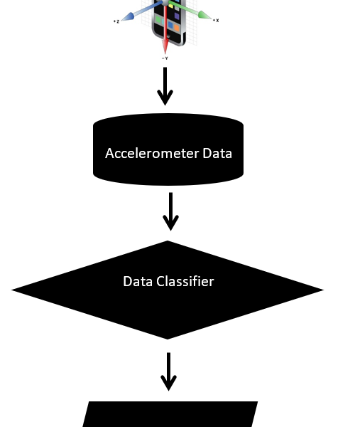
Figure 1: Block diagram of the system used for the experiments

      In this paper, we take the first step towards implementing such a system by proposing robust accelerometer data features that can distinguish between sober and intoxicated individuals. We then test these features using five Supervised Machine Learning models to see their accuracy in predicting individuals’ sobriety levels: Support Vector Machines (SVM), Decision Tree Learning, Boosting, K-Nearest Neighbors (KNN), and Neural Networks (NN) [4].

2. Related Works

Several researchers have focused their prior research on movement-pattern recognition by using accelerometers, especially since these days all mobile devices are embedded with highly accurate and precise accelerometers [5]. There have been many interesting mobile applications developed, which can detect the individuals’ activities, such as daily exercises or crossing the street, by solely analyzing the accelerometer data.

There have also been several papers that have proposed different variations of mobile systems to detect individuals’ intoxication levels:

1. Detecting abnormalities in individuals’ gaits while they walk intoxicated [6–9].
2. Evaluating eye (iris) movements of individuals who are intoxicated [10,11].
3. Monitoring the steadiness of postures of intoxicated individuals [12].

      These mobile systems can sense individuals’ intoxication levels and log the location/time of the incidents. Although these papers show the individual differences in step variance time among individuals, the differences are relative to everyone’s unique baseline, so the differences cannot be used to cleanly separate any intoxicated and sober individuals in the general population.

3. Methodology

3.1.  Physiological Basis

 One of the first symptoms that individuals exhibit as they become intoxicated is that they have decreased balance and motor coordination.  This is because of the effect of alcohol on the brain’s chemistry that it achieves by changing the neurotransmitters’ levels. These neurotransmitters are entities that act as chemical messengers, which send critical human signals throughout the body. These signals include those that control thought processes, behaviors, and emotions. Many believe that out of all the neurotransmitters, alcohol specifically targets the GABA neurotransmitter [13].

3.2.  Physical Activity Data Collection

With these factors in mind, we planned our experiments such that we could easily distinguish between intoxicated and sober subjects based on the subjects’ abilities to balance their bodies and maintain steady postures. Our proposed mobile-based system logs subjects’ accelerations along the x-, y-, and z-axes.

In order to collect the subjects’ data, we created an Android app that runs on a Motorola Moto G mobile phone. This device contains a built-in API, which outputs the device’s linear acceleration after negating the effects of gravity. Our Android app has a built-in button, which is used to start and stop data collection periods during our experiments.

For our experiments, we recruited two subjects, Subject 1 and Subject 2, to grip the mobile devices in their right hands, keep their right arms outstretched, and maintain those steady postures for 10 seconds. The subjects’ right arms form 90-degree angles with their bodies while their left arms are kept by their sides. Additionally, their right feet are in front of the left feet in straight lines, so that their left toes are touching their right heels. During the experiments, the subjects keep their eyes to better test their balance and motor skills.

We first tested both subjects in sober states, before they consumed any alcohol. After that, both subjects consumed 3, 6, and 9 drinks of alcohol over a period of 120 minutes, while we recorded their data. To keep results consistent, we defined one drink in this paper to be 1.25 oz of 80 proof liquor i.e., vodka.

4. Results

After we finished our experiments with both subjects, we had four data points per subject, which came out to eight total data points for our initial analysis. For each of the data points, we plotted the subjects’ accelerations across the x-, y- and z-axes against their times, which can be seen above in Figures 2 – 9.

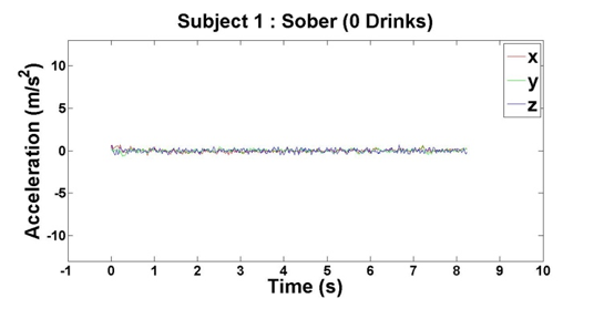
Figure 2: Accelerometer reading when Subject 1 has had 0 drinks

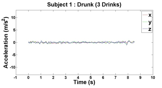
Figure 3: Accelerometer reading when Subject 1 has had 3 drinks

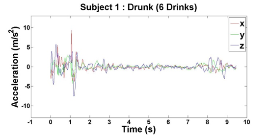
Figure 4: Accelerometer reading when Subject 1 has had 6 drinks

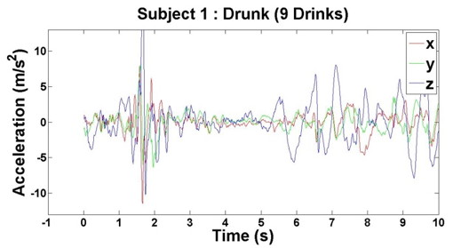
Figure 5: Accelerometer reading when Subject 1 has had 9 drinks

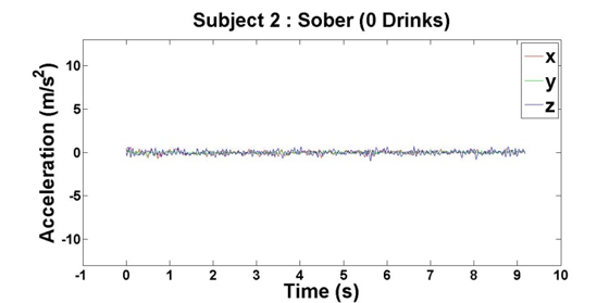
Figure 6: Accelerometer reading when Subject 2 has had 0 drinks

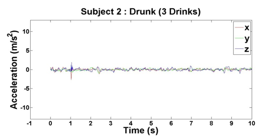
Figure 7: Accelerometer reading when Subject 2 has had 3 drinks

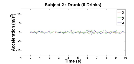
Figure 8: Accelerometer reading when Subject 2 has had 6 drinks

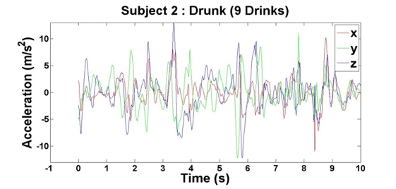
Figure 9: Accelerometer reading when Subject 2 has had 9 drinks

5. Supervised Learning Model Results

Based on the results of our experiments, we clearly see a distinction between the sober data (0 – 3 drinks) and intoxicated data (6 – 9 drinks). Additionally, there is a relationship between the number of drinks the subjects consumed and the “unsteadiness” of their corresponding data. In order to capture this change, we examined two features: variance and highest frequency.

Table 1: Tabulation of variance, highest frequency, and BAC for Subject 1

Number of Drinks	Estimated BAC	Variance	Highest Frequency
0	0	0.0382	0.1227
3	0.06	0.06059	0.11793
6	0.19	1.749063	2.860169
9	0.28	9.80903	1.5984

Table 2: Tabulation of variance, highest frequency, and BAC for Subject 2

Number of Drinks	Estimated BAC	Variance	Highest Frequency
0	0	0.0556	0.1092
3	0.06	0.06059	0.11793
6	0.19	0.214869	2.216312
9	0.28	12.0609	0.92764

The first distinguishing feature we found was the variance in the amplitude (as can be seen in Table 1). We calculated it for each axis, and then we selected the maximum variance from all the three axes. This helped make the feature more stable as the subjects held the phones in different positions, since we noticed that the variances transferred amongst the axes.

The second distinguishing feature we found was the highest frequency component of the time-series data (as can be seen in Table 2). However, the relationship was not easy to detect as in the case of the previous correlation between BAC and variance, despite the fact that the highest frequency for intoxicated data was still higher than the highest frequency for sober data.

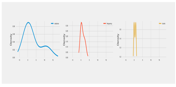
Figure 10: Breakdown of data in terms of datapoints across both subjects

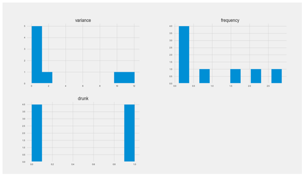
Figure 11: Density plots of the raw data for both subjects

Both the variance analysis and the highest frequency analysis were performed on Subject 1’s data and Subject 2’s data. Figures 10 – 11 given above indicate different levels of increasing variance and highest frequency, which we use to estimate the BAC of Subjects 1 and 2. The BAC is calculated using the number of drinks consumed and the body mass of each subject.

Based on these results, we tried the following Supervised Machine Learning methods to determine which methods were most effective at distinguishing between sober and intoxicated subjects, where we used Subject 1’s data as the training dataset and Subject 2’s data as the test dataset.

5.1.  SVM

For the SVM implementation, we used the Python class “sklearn.svm.SVC” [14]. For our implementation, we used two different SVM models to see the different effects on the datasets (as shown in the Table 3). First, we used the original SVM model with the values of “random_state=None, kernel=poly”. However, to see the effect of hyperparameter tuning the original SVM model, we updated several different parameters “random_state=0, kernel=rbf” [15,16].

Table 3: SVM model statistics

SVM Type	Accuracy (%)	Execution Time (s)
Default SVM	100	0.18
Adjusted SVM	67	0.19

5.2.  Decision Tree Learning

For the decision tree implementation, we used the Python class “sklearn.tree.DecisionTreeClassifier” [17]. For our implementation, we used two different decision trees to see the different effects on the datasets (as shown in the Table 4).  First, we used the regular decision tree with the default values of “gini” for the Gini impurity and “None” for the “max-depth”. However, to see the effect of pruning the trees, we tested two different parameters: setting “entropy” for the information gain and setting the “max_depth” to “3” [18].

Table 4: Decision Tree Learning model statistics

Decision Tree Type	Accuracy (%)	Execution Time (s)
Default Decision Tree	67	0.71
Pruned Decision Tree	100	0.81

5.3.  Boosting

For the decision tree implementation, we used the Python class “sklearn.tree. GradientBoost-ingClassifier” [19]. For our implementation, we used two different boosting classifiers to see the different effects on the datasets (as shown in the Table 5). First, we used regular gradient boosting with the default values of “n_estimators=100, learning_rate=0.1, max_depth=3” [20]. However, to see the effect of hyperparameter tuning the boosted model, we updated several different parameters “n_estimators=1000, learning_rate=1.0, max_depth=1” [16,18].

Table. 5. Gradient Boosting model statistics

Gradient Boosting Type	Accuracy (%)	Execution Time (s)
Default Gradient Boosting	67	1.13
Adjusted Gradient Boosting	67	1.12

5.4.  KNN

For the KNN implementation, we used the Python class “sklearn.neighbors.KNeighborsClassifier” [21]. For our implementation, we used two different KNN models to see the different effects on the datasets (as shown in the Table 6). We created a loop to test the models on our dataset by performing hyperparameter tuning and updating the “n_neighbors” value to values 2 through 8 [16,22].

Table 6: KNN model statistics

KNN Type	Accuracy (%)	Execution Time (s)
Default KNN	75	0.54
Adjusted KNN	80	0.53

5.5.  Neural Networks

For the neural network implementation, we used the Python class “keras.Sequential” [22]. For our implementation, we used two different models to see the different effects on the datasets (as shown in the Table 7). First, we used the regular keras model with two layers and 1000 epochs for the number of iterations across the data. However, to see the effect of an additional layer in my model, we tested the same keras model with a third layer and “epochs” value of “1000” for the number of cycles across the data [13,23].

Table. 7. NN model statistics

NN Type	Accuracy (%)	Epoch
Default NN	100	1000
Adjusted NN	67	1000

6. Analysis

6.1.  SVM

This algorithm gave us some of the better results in both subjects’ datasets, as can be seen in Figure 12 below. This was potentially due to the fact that this algorithm is a good general-purpose classification algorithm, especially since we used the “rbf” kernel, which is known for its general and wide-spread use across many types of datasets [24].

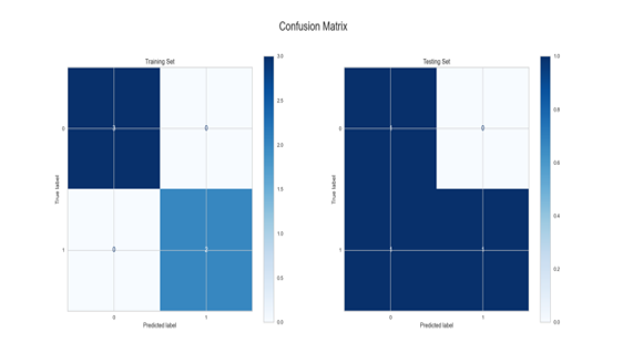
Figure 12: Confusion Matrix for SVM model

The main goal of this algorithm is to divide datasets into several classes in order to find a maximum marginal hyperplane (MMH). This can be done in the following two steps where first Support Vector Machines will generate hyperplanes iteratively that separate the classes in the best way and thereafter, they will choose the hyperplane that segregate the classes correctly [25].

We decided to perform hyperparameter tuning on our SVM and test between the rbf and polynomial kernels. We tested these because we know that the polynomial kernel is typical considered more generalized and therefore less efficient and accurate, but the rbf kernel is considered to be one of the most preferred kernel functions in SVM [24].

Based on the average runtime for our runs, we got 0.18 seconds per run as per wall clock time.

Unlike other algorithms, we didn’t do too many modifications. We only tested with different kernels, since we wanted to test a kernel that was good with generalized results to avoid overfit-ting/underfitting the long-tailed tailed variables. We didn’t show the results for the “poly” kernel because the “rbf” kernel performed better on the non-uniform datasets.

6.2.  Decision Tree Learning

We generally got better training results with decision trees, as can be seen in Figures 12 – 13 above. This might be due to our pruning methods, or it could be because of the bi-directional tails in some of the attributes in the dataset that rendered the algorithm less effective.

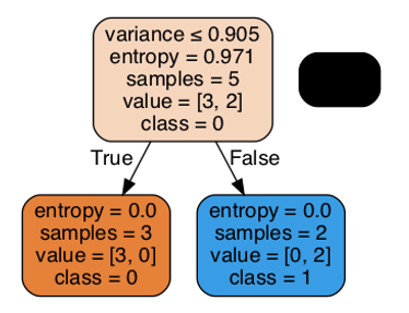
Figure 13. Node breakdown of Decision Tree model

This represents a flowchart-like tree structure, in that each internal node signifies a test on an attribute, each branch represents an outcome of the test, and each leaf node (terminal node) holds a class label [26]. This algorithm performs bests on non-linear datasets, which makes it a good choice (in theory) for our non-linear datasets

We decided to prune our trees using “criterion=entropy, max_depth=3”. We chose entropy because there are features that have “uncertainty” as they the values are clustered very close to each other [23]. Additionally, we did not want to overfit the model based on the training data, so we limited the max_depth to 3 [23].

Based on the average runtime for our runs, we got 1.12 seconds per run as per wall clock time.

As we mentioned above, we decided to prune our trees using “criterion=entropy, max_depth=3”. The results for the classifier for the default values were due to the fact that the model overfit on the training data and didn’t give as good performance on the testing data.

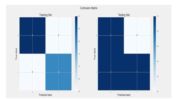
Figure 14: Confusion Matrix for Decision Tree model

6.3.  Boosting

This algorithm provided interesting results because for both datasets because the larger the training data size, the better the test predictions, as can be seen in Figures 14 – 15 below. This could be due to the fact that, similar to our neural network algorithm implementation, we used a large number of iterations.

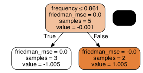
Figure 15: Breakdown for Boosting model

Since we were doing a Binary Classification problem, we used Gradient Boosting, which builds an additive model in a forward stage-wise fashion. This allows it to optimize arbitrary differentiable loss functions, where in each stage n_classes, regression trees are fit on the negative gradient of the binomial or multinomial deviance loss function [27].

We decided to perform hyperparameter tuning on our GradientBoostingClassifier and set “n_estimators=1000, learning_rate=1.0, max_depth=1”. We chose these values because we know that Boosting algorithms are prone to overfitting, so by choosing a high number of boosting stages to perform while shrinking the contribution of each tree by learning_rate, we thought we could counteract that tendency [19].

We set “n_estimators=1000”, so there were 1000 iterations per run. We decided to test with different values for “learning_rate” and “n_estimators” and only showed the results for “n_estimators=1000” and “learning_rate=1.0”, because this combination showed the best performance. This is because we can have a large “large learning rate” with iterations or have a “slow learning rate” with more iterations. This combination was a good middle choice to get the best of both parameters [24].

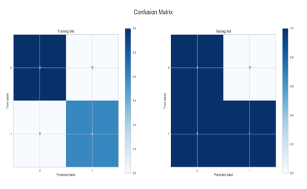
Figure 16: Confusion Matrix for Boosting model

6.4.  KNN

This algorithm gave us expected results in that as our training dataset size increased, our test performance decreased significantly, as can be seen in Figures 16-17 below. This is a clear case of the algorithm overfitting on the training dataset and suffering as a result on the testing dataset.

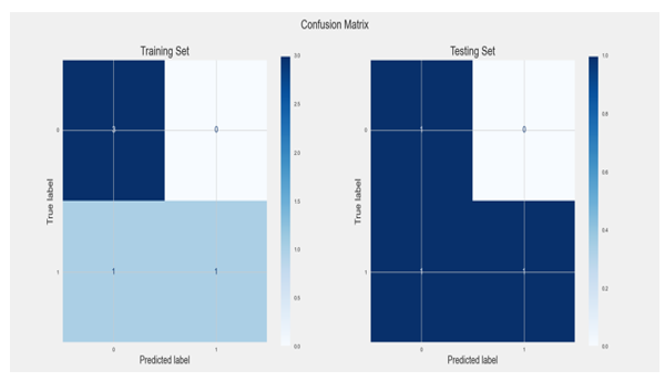
Figure 17: Confusion Matrix for KNN model

This algorithm uses the nearest neighbors in a dataset, where those data points that have minimum distance in feature space from our new data point. In this algorithm, “K” is the number of such data points we consider as part of our implementation of the algorithm. As a result, distance metric and K value are two important considerations while using the KNN algorithm [14].

We decided to perform hyperparameter tuning on our KNN model and test the k values from two through five. We tested these because we wanted to test the underfitting vs overfitting nature of our model and realized that each of the two datasets had different k values that performed the best.

Based on the average runtime for my runs, we got 0.54 seconds per run as per wall clock time.

The only tuning we did on our KNN classifier was testing the k values from two through eight. We didn’t show the results for the other values because the performance was degrading after certain “k” values for both datasets.

6.5.  Neural Networks

We noticed that this algorithm gave us the most consistent results across both datasets, as can be seen in Figure 18 below. This might be due to the large number of cycles we ran the algorithm on both datasets.

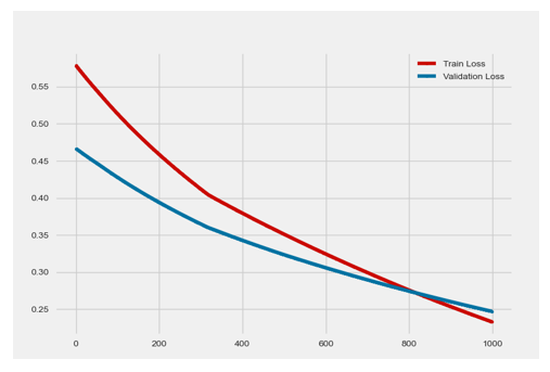
Figure 18: Loss function for NN model

This represents a mind-like algorithm which has different layers of nodes, or neurons, that get activated based on different parameters. In the case of classification datasets, like both of ours, the output layer classifies each example, applying the most likely label. Each node on the output layer represents one label. In turn, that node turns on or off according to the strength of the signal it receives from the previous layer’s input and parameters [28].

We decided to perform hyperparameter tuning on our neural networks using two activation functions: “relu” and “sigmoid”. We chose sigmoid because “the use of a single Sigmoid/Logistic neuron in the output layer is the mainstay of a binary classification neural network” [27].

We set epoch to 1000 for our tests, so there were 1000 cycles per run and we decided to test with two different stopping criteria: epoch 200 and epoch 1000. We didn’t choose to show the results for the epoch 200 because both the accuracy was higher for the epoch 1000 neural networks due to the higher number of cycles that all of the data was being processed [29]. Additionally, we tested with two and three activations layers, but only showed results for two activation layers because the adding the third activation layer hurt accuracy on the test dataset due to the fact that we used “softsign” as our third layer, which skewed results negatively [30].

7. Conclusion

The data we collected from our two subjects confirms that the effect of alcohol consumption by individuals can be strong enough to alter accelerometer readings. These readings can then be used to classify individuals’ sobriety levels. One of the limitations of our approach is that clear distinctions are mostly visible only for subjects who are well beyond the regular drinking amount, therefore, for intoxicated individuals who are not well beyond that drinking amount, the classifier model that we built is not as successful in establishing a clear difference between sober and intoxicated states. Additionally, in order to be able to classify “less intoxicated” vs “more intoxicated”, we will require larger and more diverse datasets.

7.1.  Effect of Cross-Validation

There is tremendous benefit to use a K-folds cross-validation over the standard random data splits because when we build K different models, we are able to make predictions on all of our data. This is especially helpful in smaller data sets so that the algorithm can recognize better patterns [24].

7.2.  Definition of Best

For our analysis, we defined “best” as the algorithm that gave us the best balance of the highest test accuracy (not necessarily highest training accuracy) based on a training set size and the fastest execution time.

7.3.  Best Classifier

Each algorithm has its own strengths and weaknesses and is therefore good/bad on different types of datasets. That being said, we saw that for datasets that contain both uniform and tailed distributions, such as our subjects’ accelerometer data, the Decision Tree Learning was the best Supervised Machine Learning method and should be used as part of our mobile device sobriety classification system.

8. Future Work

In order to build on our research, we want to address the issue of limited test subjects and expand the experiments to include a larger sample size that is comprised of individuals with varied genders, body compositions, backgrounds, etc. [31].

Additionally, we want to explore real world-use cases that can be addressed by our research results. For example, our system can be used with data from any accelerometer, such as those found in car steering wheels. This means that if our system is embedded into cars, then cars’ internal systems will potentially be able to warn drivers if their BAC levels are above the legal driving limit, which will directly reduce traffic fatalities caused by alcohol consumption.

Conflict of Interest

The authors declare no conflict of interest.

Acknowledgment

We owe our gratitude to our mentors for guiding us throughout our experiments: Professor Pei Zhang and Dr. Xinlei Chen. We also thank both of our anonymous subjects for participating in our experiments, so that we could monitor their data and use it as part of our analysis.

1. D. Kumar, A. Thanikkal, P. Krishnamurthy, X. Chen, P. Zhang, “Accelerometer-Based Alcohol Consumption Detection from Physical Activity,” in 2021 17th International Conference on Wireless and Mobile Computing, Networking and Communications (WiMob), 415–418, 2021, doi:10.1109/WiMob52687.2021.9606257.
2. R.W. Olsen, H.J. Hanchar, P. Meera, M. Wallner, “GABAA receptor subtypes: the ‘one glass of wine’ receptors,” Alcohol, 41(3), 201–209, 2007, doi:https://doi.org/10.1016/j.alcohol.2007.04.006.
3. Alcohol Facts and Statistics. National Institute on Alcohol Abuse and Alcoholism, 2021, Online: http://www.niaaa.nih.gov/alcohol-health/overview-alcohol-consumption/alcohol-facts-and-statistics..
4. D. Kumar, Supervised Learning, Georgia Institute of Technology, 2022.
5. R. Li, G.P. Balakrishnan, J. Nie, Y. Li, E. Agu, K. Grimone, D. Herman, A.M. Abrantes, M.D. Stein, “Estimation of Blood Alcohol Concentration From Smartphone Gait Data Using Neural Networks,” IEEE Access, 9, 61237–61255, 2021, doi:10.1109/ACCESS.2021.3054515.
6. C. Nickel, C. Busch, “Classifying accelerometer data via hidden Markov models to authenticate people by the way they walk,” IEEE Aerospace and Electronic Systems Magazine, 28(10), 29–35, 2013, doi:10.1109/MAES.2013.6642829.
7. B. Suffoletto, P. Dasgupta, R. Uymatiao, J. Huber, K. Flickinger, E. Sejdic, “A Preliminary Study Using Smartphone Accelerometers to Sense Gait Impairments Due to Alcohol Intoxication,” Journal of Studies on Alcohol and Drugs, 81(4), 505–510, 2020, doi:10.15288/jsad.2020.81.505.
8. S. Bae, D. Ferreira, B. Suffoletto, J.C. Puyana, R. Kurtz, T. Chung, A.K. Dey, “Detecting Drinking Episodes in Young Adults Using Smartphone-Based Sensors,” in Proc. ACM Interact. Mob. Wearable Ubiquitous Technol., Association for Computing Machinery, New York, NY, USA, 2017, doi:10.1145/3090051.
9. J.A. Killian, K.M. Passino, A. Nandi, D.R. Madden, J. Clapp, “Learning to detect heavy drinking episodes using smartphone accelerometer data,” CEUR Workshop Proceedings, 2429, 35–42, 2019.
10. T.H.M. Zaki, M. Sahrim, J. Jamaludin, S.R. Balakrishnan, L.H. Asbulah, F.S. Hussin, “The Study of Drunken Abnormal Human Gait Recognition using Accelerometer and Gyroscope Sensors in Mobile Application,” in 2020 16th IEEE International Colloquium on Signal Processing & Its Applications (CSPA), 151–156, 2020, doi:10.1109/CSPA48992.2020.9068676.
11. Z. Arnold, D. Larose, E. Agu, “Smartphone Inference of Alcohol Consumption Levels from Gait,” in 2015 International Conference on Healthcare Informatics, 417–426, 2015, doi:10.1109/ICHI.2015.59.
12. Aiello, Agu, “Investigating postural sway features, normalization and personalization in detecting blood alcohol levels of smartphone users,” in 2016 IEEE Wireless Health (WH), 1–8, 2016, doi:10.1109/WH.2016.7764559.
13. W. S, How Alcoholism Works, HowStuffWorks Science, 2021, Online: http://science.howstuffworks.com/life/inside-the-mind/ human brain/alcoholism4.htm
14. Sklearn.svm.SVC, Scikit, 2021, Online: https://scikit-learn.org/ stable/modules/generated/sklearn.svm.SVC.html
15. A Beginner’s Guide to Neural Networks and Deep Learning, Pathmind, 2021, Online: https://wiki.pathmind.com/neural-network#logistic
16. R. Pramoditha, Plotting the Learning Curve with a Single Line of Code.” Medium, Towards Data Science, Medium, Towards Data Science, 2021, Online: https://towardsdatascience.com/plotting-the-learning-curve-with-a-single-line-of-code-90a5bbb0f48a
17. Sklearn.tree.decisiontreeclassifier, Scikit, 2021, Online: https://scikit-learn.org/stable/modules/generated/sklearn.tree. Decision TreeClassifier.htmll
18. Romuald_84, Boosting: Why Is the Learning Rate Called a Regularization Parameter?” Cross Validated, Cross Validated, 1963, Online: https://stats.stackexchange.com/questions/168666/boosting -why-is-the-learning-rate-called-a-regularization-parameter..
19. Sklearn.neighbors.kneighborsclassifier, Scikit, 2021, Online: https://scikit-learn.org/stable/modules/generated/sklearn.neighbors. KNeighborsClassifier.html.
20. Baeldung, Epoch in Neural Networks, Baeldung on Computer Science, 2021, Online: https://www.baeldung.com/cs/epoch-neural-networks.
21. C. Chaine, Using Reinforcement Learning for Classfication Problems, Stack Overflow, 1965, Online: https://stackoverflow.com/questions/44594007/using-reinforcement-learning-for-classfication-problems.
22. Htoukour, Neural Networks to Predict Diabetes, Kaggle, 2018, Online: https://www.kaggle.com/htoukour/neural-networks-to-predict-diabetes
23. Alcohol’s Effects on the Body. National Institute on Alcohol Abuse and Alcoholism, NIH, 2021, Online: http://www.niaaa.nih.gov/alcohol-health/alcohols-effects-body
24. Sklearn.ensemble.gradientboostingclassifier, Scikit, 2021, Online: https://scikit-learn.org/stable/modules/generated/sklearn.ensemble. GradientBoostingClassifier.html.
25. Shulga, Dima, 5 Reasons Why You Should Use Cross-Validation in Your Data Science Projects, Medium, Towards Data Science, 2018, Online: https://towardsdatascience.com/5-reasons-why-you-should -use-cross-validation-in-your-data-science-project-8163311a1e79.
26. Decision Tree, GeeksforGeeks, 2021, Online: https://www.geeksforgeeks.org/decision-tree/
27. Decision Tree Algorithm – A Complete Guide, Analytics Vidhya, 2021, Online: https://www.analyticsvidhya.com/blog/2021/08/ decision-tree-algorithm/.
28. Complete-Life-Cycle-of-a-Data-Science-Project, Complete Life Cycle Of A Data Science Project, 2021, Online: https://awesomeopensource.com/project/achuthasubhash/Complete-Life-Cycle-of-a-Data-Science-Project
29. Machine Learning with Python – Algorithms, 2022, Online: Online: https://awesomeopensource.com/project/achuthasubhash/Complete-Life-Cycle-of-a-Data-Science-Project
30. K. Team, Keras Documentation: The Sequential Class, Keras, 2021, Online: https://keras.io/api/models/sequential/
31. D. Deponti, D. Maggiorini, C.E. Palazzi, “DroidGlove: An android-based application for wrist rehabilitation,” in 2009 International Conference on Ultra Modern Telecommunications & Workshops, 1–7, 2009, doi:10.1109/ICUMT.2009.5345442.

(Click Here)