1. Introduction

The world has recently witnessed a great revolution in the way information is transmitted from one place to another. Wireless communication has advanced from mere point-to-point communication to becoming a viable tool to facilitate economic development, security enhancement and reliable public service delivery. The basic task for a communication system is to reliably deliver information from the source to the destination, using a transmitter and a receiver across a channel. The performance of conventional communication techniques is seen limited in operation and are sub-optimal due to the challenges which present themselves in the form of latency, reliability, energy efficiency, flexibility etc [1]. The fast emergence of many unprecedented services such as artificial intelligence, smart homes, factories and cities, wearable devices for physical challenged, robots, autonomous vehicles, big data, internet-of-things etc. are challenging the conventional approaches and mechanisms to communication. Recent research and technology advancements have contributed to an enviable progress in developing novel and enhanced mechanisms in the layers of communication system. Despite that, more research is on the progress in providing optimal performance for wireless communication networks.

It is important to note that emerging wireless communication systems typically transmit high data rates to provide wide range of services for better voice quality, improved data, images and other multimedia applications. Conversely, during wireless signal propagation, the systems usually encounter channel impairments, resulting in data errors at the receiver end. To correct this, requires adequate error correction codes to detect and correct symbol errors during transmission.

The introduction of Joint Source-Channel Coding (JSCC) technique in wireless communication has been able to address most of the challenges that are inherent in the separation-based schemes, (i.e., the conventional two-step encoding process for the image/video data transmission, source coding and channel coding) [2]. Recently, it became a considerable research topic in communication systems and information technology, with the application in areas like audio/video and satellite transmission, as well as in space exploration. Despite the successes recorded by JSCC techniques, it still encounters some performance flaws inherent in its fundamental assumptions that could prove very costly for modern communication systems. This flawed assumption ripples through the design of systems based on conventional JSCC techniques in the form of increased processing and algorithmic complexity to combat noise in its various forms and also cater for additive information. This complexity can introduce a certain level of latency which is detrimental to the actualization of low latency systems. Furthermore, other inherent limitations include inability to fulfil bulky data and very high-rate communication requirements in multifaceted conditions as seen in most complex channel models. Others include; in low latency communication systems, in rapid and reliable signal processing application and in limited and sub-optimal block structures, due to the fixed block configuration of the communication system etc [1]. However, the recent introduction of Deep Learning (DL) technique and its fundamental based autoencoder concept, characterized with its simplicity in implementation, flexibility and ability in adapting to complex channel models, has been able to handle most of the complexities due to the stated advantages it possesses [1]. It has recently been successfully applied in solving various real-life applications such as in pattern recognition, speech and language processing, media entertainment, medicine, biology and security systems. DL is quite robust and scalable in application.

Deep learning is a subset of Machine Learning (ML) that exhibits greater potentials in building complex concept from simpler concepts.  It has useful tools to process ultra-high data and shows high performance accuracy in recognition and prediction. Deep learning algorithm is seen to outperform machine learning algorithm, especially in handling difficult and complex  tasks such as in image and voice recognition, it is considered to be more valuable in cases where needful reduction in  computational complexities and overhead processing are preferred. Deep learning tends to rely on its intelligence to define its own finest features, it does not require humans to perform any feature-creation activity. Among the existing DL models, Deep Neural Networks (DNNs) are considered to be the most known model, other deep architectures such as  Neural Processes(NPs), Deep Gaussian Processes (DGPs) and  Deep Random Forests (DRFs) could be categorized as deep models made up of multiple layered structures [1,3].

Based on the research motivations, the study focuses on implementing JSCC using DL approach without the need for explicit codes. The study aims to develop a Deep Neural Network (DNN) symbol models for JSCC in an end-to-end pattern. Python/Keras and TensorFlow backend are simulation tools used to evaluate the error correction performance and data reconstruction. Bit Error Rate (BER) and Block Error Rate (BLER) are the selected parameters for the system analysis. Simulations were carried out to perform the BER/BLER and its reliability compared to the conventional communication approach with preference in reducing the processing complexity and latency. The performance analysis of the developed deep joint source-coding algorithm with different Signal-to-Noise Ratio (SNR) values were also evaluated.

In our study, the motive is to extend the preceding study on autoencoder-based end-to-end learning of communications system, evaluate its characteristic performance in varying system configurations and also realize the potentials of autoencoder-based end-to-end learning mechanisms for communications systems.

1.1    Model of A Simple Communication System

A typical communication system in its most fundamental form consists of a transmitter, channel, and receiver as illustrated in figure1. The communication system facilitates the transfer of information signal from one point to another through a process that involves three basic stages; coding, mapping and decoding. Firstly, the information signal is encoded into a message x of block length k. Each message x can be represented in the block length  k =  number of bits. The transmitter can transmit any of the acceptable messages out of M possible messages x ∈ M = {1, 2, …, M} of block length k through n discrete users of the allocated communication channel. The transmitter on the other hand, performs the mapping f_θ:  →  [4]. A vector g of n complex symbols is transmitted across the channel to facilitate the sending of the message x to the receiver[1]. The presence of noise in the channel causes signal distortions to the transmitted symbols.  The receiver stage is concerned with mapping the transmitted signal to the receiver. The mapping of the transmitted signal is actualized using the transformation g_?:  → , portraying the fact that the decoding function inverts the operation of the encoding function. At the receiving end, as the signal is intercepted by the receiver, that is the signal  i ∈  , the receiver generates the estimate  of the originally transmitted message x.  Figure 1 shows the structure of a simple communication system which could be modelled using an autoencoder. A communication system can in its simplest term be described as an autoencoder that tries to reconstruct the transmitted message at the receiver as accurately as possible with the least possible errors[1]. For clarity sake, we can further describe the encoder function of the autoencoder as the transmitter  block while the decoder function as the receiver block of the system. A block diagram of an autoencoder is represented in figure 2.

From figure 2, the encoder attempts to transform the input value  into a low dimensional latent vector  . The latent vector is usually characterized of low dimension with a

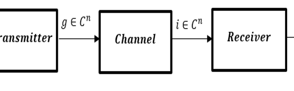
Figure 1:  Block diagram of  a Communication System

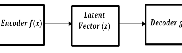
Figure 2: A block diagram representing an Autoencoder

compressed representation of the input distribution. The decoder in contrast, tries to recover the input signal from the latent vector, g\left(z\right)=\widetilde{x} . The expectation should be that the output recovered by the decoder could only approximate the input (i.e. making \widetilde{x}\ as close as possible to x)[5]. The variations between the input and the output is measured as a loss function. It is necessary to note that both the encoder and the decoder are non-linear functions.

2. Related Works

In recent years, DL-based techniques were introduced for different processing blocks of the wireless communication systems as substitutes to conventional applications such as modulation recognition[6], channel encoding and decoding[7,8], and channel estimation and detection [9–11], owing to the development of DL algorithms and system architectures.

Authors of [1], investigated the DL-based end-to-end communications performance models when deployed in a single user communication network under an Additive White Gaussian Noise (AWGN) channel. An autoencoder-based end-to-end communications system was implemented in the system validation. In[12], considered the challenges of JSCC of text /structured data using deep learning approach from natural language processing over noise channel. Their proposed technique is said to have an edge over  the existing distinct source and channel coding, particularly in scenarios when a smaller number of bits were used in describing each sentence. Their scheme achieved lower word error rates from the developed deep learning-based encoder and decoder system. The developed system uses a fixed bit length for enconding sentences of different length. This was observed to be a major drawback of their algorithm.

The authors of[13], proposed the use of neural networks to address the design of systems with block length when k =1. In [14], used simple neural network architecture in encoding and decoding of Gauss-Markov sources over additive white Gaussian noise channel. Authors of [15,16], proposed neural network for signal compression devoid of a noisy channel (i.e. only source coding), where image compression algorithms were developed using RNNs. In[17], used neural networks, in particular, Variational Autoencoders (VAEs) to design neural network based Joint Source Channel Coding and extended the system design to where k ≠1. However, their performance was reasonable but a lot was required to improve upon their performance in order to meet up with  the benchmark set by[18] . The authors of,[18] developed a new scheme for JSCC of Gaussian sources over AWGN channels. VAEs was implemented in their design but with a novel encoder architecture for the VAE specifically developed for zero-delay Gaussian JSCC over AWGN channels, a situation where the source dimension (m) is greater than the channel dimension (k). Their proposed scheme was able to improve on works of [17] with about 1dB.

Our study therefore seeks to evaluate the performance of Bit Error Rate in wireless networks using Deep Neural Network (DNN) system model for joint source channel coding in an end-to-end manner without the need for explicit codes to provide error correction. The approach is envisaged to minimize the block length of transmitted data with maximal utilization of bandwidth, increased data rate and power efficiency. Simulation models such as Python/Keras and TensorFlow backend will be implemented to oversee the process of error correction improvement and data reconstruction.

3. Method

The proposed deep learning approach for JSCC is implemented by simulation in Keras using Tensor Flow as its backend. TensorFlow provides a robust environment, creating a relatively easy-to-use package. A model is trained to mimic the conventional end-to-end communication system under certain conditions and constraints. The trained model is then tested against random data under varying conditions to determine its performance in practical scenarios.

3.1.  Autoencoder Implementation for the Proposed Scheme

An autoencoder’s main objective is to actualize a compressed representation of a given input data. An autoencoder is a neural network architecture, comprised of two distinct units; Encoder and Decoder functional units. The encoder unit primarily converts the input data into a different representation while the decoder unit

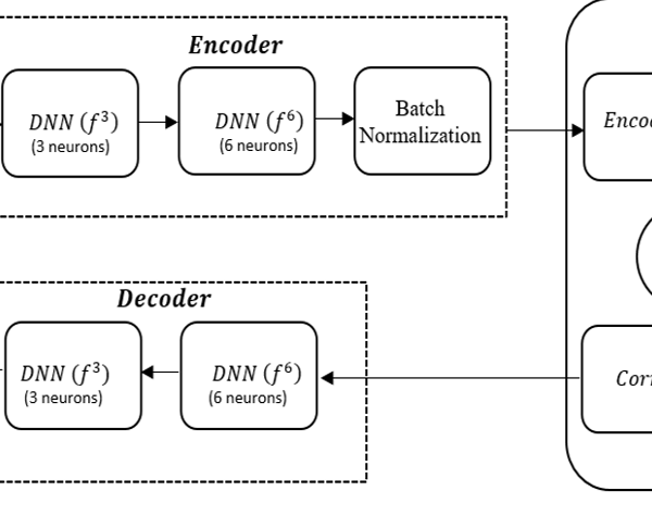
Figure 3: The FCNN Autoencoder Block Diagram

converts the new representation back into the original format, trying to recover the input data. The input data could be in different configurations such as in speech, text, image or video format. Figure 3 represents the functional block diagram of a Fully Connected Neural Network (FCNN) autoencoder.

To illustrate the performance characteristics of the deep JSCC scheme, the functional block diagram of the Fully Connected Neural Network in Fig. 3 is implemented in our simulation.  The autoencoder in this context was implemented as a fully connected feedforward Neural Network, enabled to propagate the information realized from the input, through a sequence  of non-linear transformations to get to the output.

  The autoencoder models is assumed to have undergone training for a predetermined message size (M) with its accompanying communication rate. We have two hidden feedforward DNN layers situated at the encoder end as shown in Fig.3. The first layer is  having 3 neuros while the second layer is which constitute 6 neurons. It is designed in such a way that the output of the first layer feeds into the input of the second layer etc. The two-layer blocks are connected to the batch normalization layer as represented. The batch normalization layer is introduced in the representation to satisfy the average power constraint.  An activation function known as Rectified Linear Activation Unit (ReLU) was employed by the convolutional layers (each dense layer) in order to apply nonlinearities to the model. A SoftMax activation function was implemented at the output layer in order  to output the probability distributions for each of the output category. We used the Gaussian noise layer to simulate an additive white Gaussian noise channel which in this case is represented as the noise layer.

The autoencoder is trained at full length over the stochastic channel model. The Stochastic Gradient Descent (SGD) method of optimization is used and the Adam optimizer is the preferred choice for the optimizer. The Adam optimizer’s learning rate is set at 0.001. The steps taken to select the energy per symbol to noise ratio (E_b/No) values for the AWGN channel during training are shown thus:

1. Training was done at a fixed E_b/N₀ value, 0 dB and 8 dB in this case.
2. Testing of the trained model using random E_b/N₀ values picked from a predetermined E_b/N₀ range for each training epoch. This is done to determine the BER performance during varying channel conditions.

• The testing is initiated using a higher E_b/N₀ value which decreases gradually along training epochs. In the case of the 8 dB training value, the test starts from 8 dB and is reduced by 2 dB after every 10 epochs.

We applied autoencoder model for our training and testing analysis in Keras using the TensorFlow application as its default tensor backend engine. The model was trained for  fifty (50) epochs using  sixty thousand (60,000) images, generated randomly with E_b/N₀ values for Additive White Gaussain Noise (AWGN) channel in the model training. The BER performance for the 0dB and 8dB were then compared with the Hamming code utilizing a BPSK modulation scheme.

The Bidirectional Long Short-Term Memory (BLSTM) autoencoder is also trained and tested in this simulation. It exhibits a parallel architecture to FCNN autoencoder, though, it has dissimilar structural components as shown in figure 4.

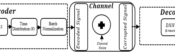
Figure 4:The BLSTM autoencoder Block diagram.

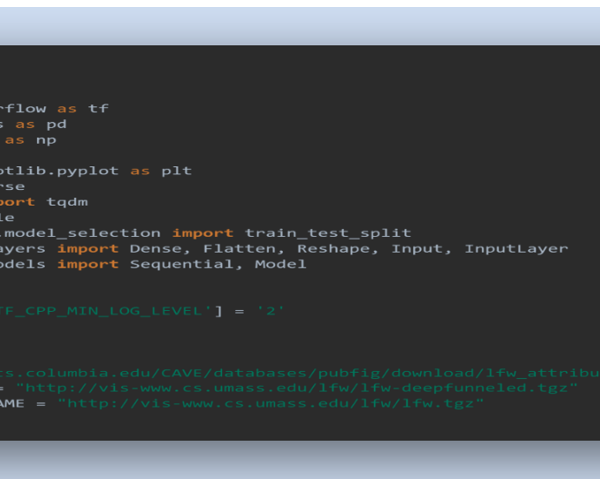
Figure 5:  Snapshot of FCNN generated codes showing imports

In figure 4, the encoder with a BLSTM has its dimension of the hidden units set to 32, while 32 refers to the number of features in each input sample. The BLSTM cell comprise of seven (7) hidden states units. In the context, each input character or element is linked to each neuron in the hidden layer. The product of the input feature and the size of the hidden layer is evaluated as the total number of connections established. The time distributed layer at the encoder section is introduced to help in flattening the output from the previous layer. At the decoder unit is implemented with a DNN layer constituting 8 neurons.

3.2 Deep Learning Algorithm for Fully Connected Neural Network (FCNN) Model

The basic steps followed to train and test the designed model in section 3.2 are highlighted as follows:

1. The imports for the model are specified. A snapshot of the code in figure 5 shows that lots of TensorFlow modules were imported. The snapshot also showed that the Labelled Faces in the Wild (LFW) dataset was utilized to train the model.
2. The dataset was loaded from its location on the internet and normalized. This entails converting the raw matrix into an image and changing the color system to RGB. The screenshots of the system functions are shown in figures 6 and 7.

Figure 6: Snapshot of function that converts raw matrix to image

Figure 7: Snapshot of function that loads LFW dataset.

Figure 8: Snapshot of dataset normalization

The images could have large values for every pixel from 0 to 255 range. Usually, in ML, the focus is to make sure the values are small and concerted around 0. This concept adopted enabled  our model to train faster with optimal results. This task is achieved through normalization of the dataset as shown in figure 8.

The dataset was split into training and test data sets. The training data is used in building the autoencoder. The algorithm for this is shown in figure 9.

1. The model was compiled in order to enable us train the model. The optimizer and loss function are specified in this stage. Figure 10 shows a snapshot of the algorithm used to accomplish the task
2. A summary of the model was generated to inspect the model in greater detail. The generated model summary is shown in figure 11.
3. Finally, the model was trained and tested by simulating practical channel conditions. Noise was introduced into the model prior to testing the model. Figure 12, shows the function used to introduce noise into the model while figure 13, shows the algorithm for training of the model at a set SNR.

The result for the simulation over 50 epochs is captured in figure 14.

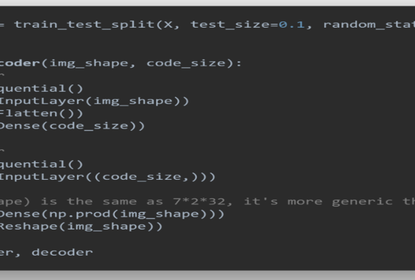
Figure 9:  Snapshot of algorithm for building the FCNN autoencoder

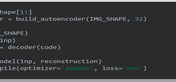
Figure 10:  Snapshot of algorithm for compiling model

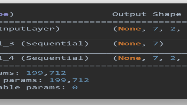
Figure 11:  Snapshot of FCNN model summary

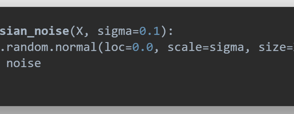
Figure 12: Snapshot of algorithm to introduce noise into the FCNN model

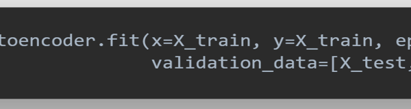
Figure 13: Snapshot of algorithm to train the FCNN model

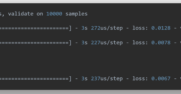
Figure 14. Snapshot of training results for the FCNN model

The steps to implement the algorithm for the LSTM and BLSTM autoencoder follow the same process and pattern that had earlier been elaborated. The only key difference is the introduction of state in the LSTM and BLSTM.

3.3 Performance Measure

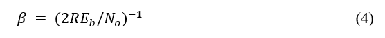
 The model was trained using the mean squared error (MSE) and categorical cross-entropy. The MSE together with two other error metrics were used to give an insight into the performance of the model. The average mean squared-error between the original input image  and reconstruction  at the output of the decoder is taken to be the loss function[2]. The loss function is given as[2]:

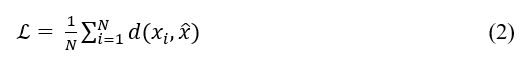
Where  =  is the mean squared-error distortion and N = 7 in the simulation. This represents the distance apart the approximation is far from the original input.  The other two error metrics factored into the simulation are the Bit Error Rate (BER) and the Block Error Rate (BLER) on channels with 0.0 dB and 8.0 dB Eb/No respectively. The BER is the number of bit errors divided by the total number of transferred bits during a studied time interval (https://en.wikipedia.org/wiki/Bit_error_rate). Bit errors in this context is simply the number of bits that are incorrectly reconstructed. Block Error Rate (BLER) refers to as the ratio of the number of blocks with error to the total number of blocks transmitted on a digital circuit. BER is affected by several factors including noise in the channel, code rate and the transmitter power level. The BLSTM autoencoder model was simulated and compared with the Hamming codes for soft and hard decoder.

The code rate R is given as[19]:

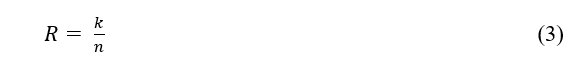
where k refers to the number of bits at the encoder input and n is the number of bits at the encoder output. The variance of additive white Gaussian noise is given as[19]:

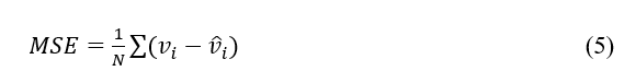
The Mean Square Error (MSE) is the variance around the fitted regression line at the decoder. It could also be referred as the Euclidean distance between the reconstructed vector  and the input vector  and indicates the distance apart the approximation is from the original input. The MSE which could be refered to as an example of a loss function is represented in equation 5[4].

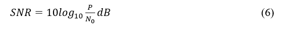
To evaluate the reconstruction accuracy of the deep JSCC algorithm in a noisy channel, an additive white Gaussian noise is modelled in the system. The average power constraint, P, is set to one (i.e. P = 1), and vary the channel SNR by varying the noise variance N₀. The channel SNR is computed as[20]:

The performance of the deep JSCC algorithm is measured in terms of the Peak Signal-to-Noise Ratio (PSNR) of the reconstructed images at the output of the decoder, defined as follows[20]:

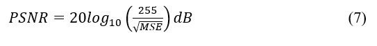
All simulations were conducted on 24-bit depth RGB images (8 bits per pixel per color channel), thus, maximum power signal is given by

 4. Simulation Results

The performance of the JSCC for wireless image transmission were evaluated using computer simulations. Simulation results of the JSCC using neural networks were based on the bit error rate (BER) performance over a range of signal-to-noise ratios. The results of the simulations were captured and displayed using graphical plots of errors versus epoch units (the number of passes through the complete dataset) for a given SNR value.

Figures 15 and 16 showed the training and test error results for the fully connected neural network autoencoder models trained on channels with 0.0dB and 8.0dB respectively. We trained the models using 60,000 samples of data, tested on 10,000 samples. Checkpointing, a fault tolerance technique for long running processes was used to retain the model state that yielded the best loss. It is an approach where a snapshot of the state of the system is taken in case of system failure.

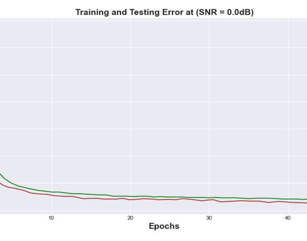
Figure 15: Bit Error Rate vs Training Epochs  for FCNN Autoencoder at (SNR= 0.0 dB) channel.

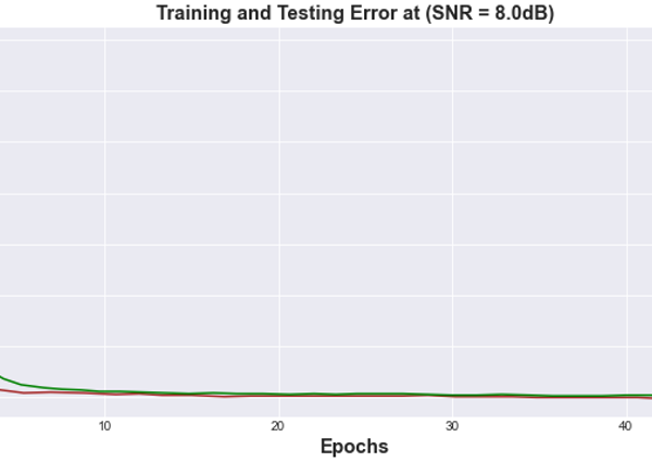
Figure 16: Bit Error Rate vs Training Epochs  for FCNN Autoencoder at  (SNR= 8.0 dB) channel

Figures 17 and 18 represent the error results from the training/test for the BLSTM Autoencoder model for SNR of 0dB and 8 dB respectively. From the graphical representation, it was observed that BLSTM autoencoder converges at a bit faster rate compare with the FCNN and appears to have a better solution to the problem of effective input reconstruction.

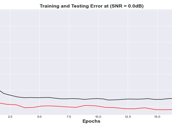
Figure 17:  Mean Squared Error vs Training Epochs for BLSTM Autoencoder at (SNR= 0.0 dB) channel

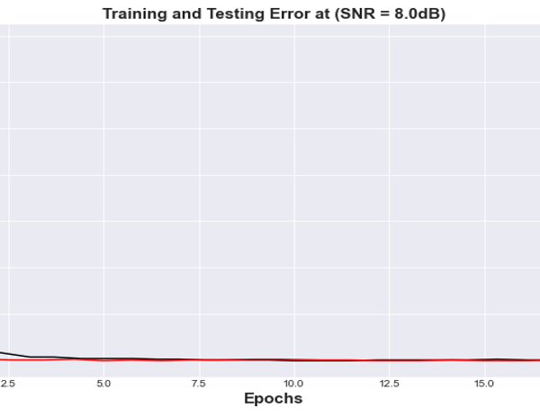
Figure 18: Mean Squared Error vs Training Epochs for BLSTM Autoencoder at (SNR= 8.0 dB) channel

4.1 Discussion

The simulated results shown in section 4, highlighted the robustness of the proposed coding scheme to various channel conditions. Figures 15-18 illustrate the number of errors in the reconstructed images versus the number of Epoch units for two different SNR values of the AWGN channel. Each curve in the figure is obtained by training the end-to-end system using a specific channel signal to noise ratio value. The performance of the learned encoder/decoder parameters on the 10,000 test images for slightly varying SNR value due to varying channel conditions were also evaluated. When the SNR_test  is  less than the SNR_train, our deep Joint Source Channel Coding algorithm is seen to demonstrate a robust scheme performance over channel deterioration and failed to experience recurrent cliff effect observed in digital systems, where the quality of the decoded signals experience nongraceful degradation whenever the SNR_test drops below a critical value close to the SNR_train. The deep JSCC design performance is more tolerable with a better stable state in the presence of channel fluctuations and exhibits a graceful degradation as the channel deteriorates. The performance is due to the autoencoder’s potential to map analogous images to nearby points in the channel’s input signal space.  On the other hand, when SNR_test is said to increase above SNR_train, a gradual improvement is observed in the quality of the reconstructed images. It is important to note that the performance in the saturation region is obtained majorly by the level of compression realized during the training phase for a given value of SNR_train.

 4.1.1 Deep Learning JSCC Versus Hamming Code

The deep JSCC algorithm is compared with the channel uncoded BPSK and Hamming code. A version of the (7,4) hamming code was implemented in the study as a measure for the experimental simulation comparison as shown in figure 19.

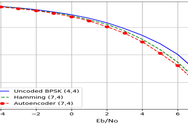
Figure 19: Bit Error Rate  for BPSK in AWGN Channel Hamming Code and Autoencoder

Figures 20 and 21 represent the comparison of the BER and BLER respectively with Hamming code and uncoded BPSK. It can be observed that, the binary long short-term memory autoencoder (BLSTM) exhibited a slight match with the Hamming code in terms of performance. The BLSTM autoencoder was able to learn the proposed joint-coding scheme by leveraging its non-linearity property. This is in direct contrast with the Hamming code which relies on a linear transformation.

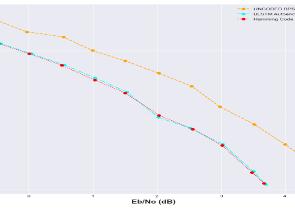
Figure 20: BER Performance comparison with Hamming code and Uncoded BPSK

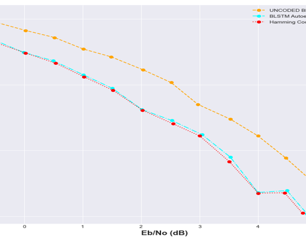
Figure 21: BLER performance comparison with Hamming code and Uncoded BPSK

From figure 20, it could be seen that autoencoder BER performance demonstrated better performance than the uncoded BPSK over the full Eb/No deployed. Hamming code implementation was closely matched by the autoencoder BER performance. It can also be observed from figures 20 and 21 that, the BLSTM configuration have almost a matched BER performance across the full E_b/N₀ range. The performance is very phenomenal owing to the fact that Hamming code is just a channel coding technique. It can also be observed from figure 20 that as the SNR improves, the BLSTM gets closer to matching the Hamming code in terms of BER performance.

4.1.2 Comparison of Bit Error Rate Performance

Figures 22-24, show the BER performance of BPSK coding schemes and the implementation of convolution code at 1/2 and 1/3 code rate and the uncoded systems respectively. When comparing the results with the results obtained from simulations of deep learning JSCC algorithm for various models, it can be observed that the convolutional codes have a similar BER performance to the deep learning JSCC based systems implemented in the study. However, as can be deduced from figure 20, the deep learning JSCC algorithm for the optimized BLSTM model was slightly better than the convolution code for R=1/3 in figure 22 and also with an improved performance over the convolution code for R=1/2 in figure 23. Under adverse channel conditions (SNR = 0), the BLSTM has a BER far lower than the convolutional codes for  ,   and the uncoded system. This shows that the autoencoder outperforms the the convolution codes.

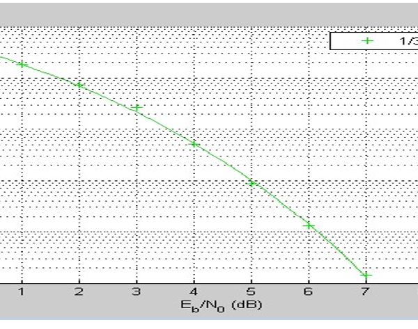
Figure 22: Result showing the Convolution Code for 1/3

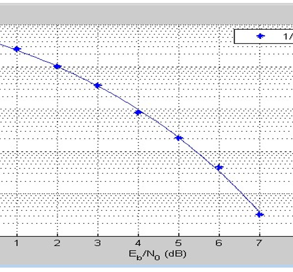
Figure 23:  Result showing the Convolution Code for 1/2

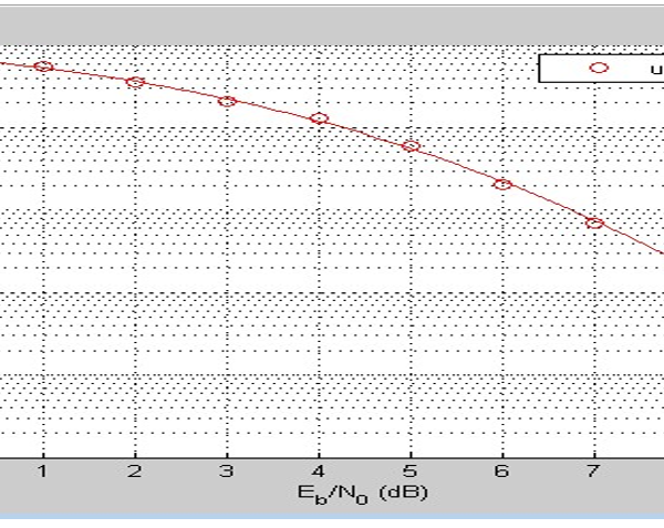
Figure 24: Result showing the uncoded system

4.2 Significance of Results

The results illustrated in figures 15-18, demonstrate the robust performance of the proposed deep learning JSCC algorithm. These results showed that the proposed algorithm has an acceptable BER performance without the need for explicitly specified codes. The comparative analyses results in figures 20 and 21 illustrated that, the BLSTM autoencoder exhibits robustness and performs favorably when compared with the Hamming code with different values on channel SNR. Owing to the fact that the autoencoder-based system does not require input block sizes of a larger dimension to operate as the input size to the model[1], it still has the capacity to achieve an acceptable BER performance with only k bits  at k = 8,  which exhibits quite a small block size length in comparison with the existing systems that usually operate within the range of 100s to 1000s bits long block sizes[19]. A system that exhibits such performance would be preferable, and stand a good characteristic advantage for low latency and low throughput communication systems. In such scenario, it is believed that short message transmission is possible to achieve even at a very low error rate, with minimal computational and processing complexities and delay response compare with the existing technique(s)[19]. This could also reduce the transmitter or antenna cost, with improved data rates for the same transmitter power and antenna size.

5. Conclusion

The study was primarily aimed at providing an improved channel performance approach for wireless communication network. The study sought to achieve this aim by focusing on improving the BER performance, reducing latency and the processing complexity in Joint Source Channel Coding systems. The study implemented a deep learning algorithm to enhance on the limiting performance of the conventional systems.

The Deep learning autoencoder system models were applied as an equivalent to existing models. The hamming and convolution codes in addition to the uncoded system were carefully analyzed with deep learning autoencoder models. The deep learning autoencoder model demonstrated a performance that compared favorably with the hamming code and better than the convolution codes, and uncoded systems. The results obtained showed that the autoencoder model exhibits better and or approximately equal BER performance even when hamming code (soft decoding) was utilized.

Further studies could be focused towards exploiting more advanced deep learning architectures and models in the autoencoder that could further enhance the compression performance of data with minimal BER.

Conflict of Interest

The authors declare no conflict of interest.

Acknowledgment

The authors extend their appreciation to Federal University of Technology, Owerri for providing the enabling environment for learning and to all the colleagues that contributed in various ways towards the success of the research study.

1. R.N.S. Rajapaksha, “Master’s Thesis: Potential Deep Learning Approaches for the Physical,” (July), 1–59, 2019.
2. E. Bourtsoulatze, D. Burth Kurka, D. Gunduz, “Deep Joint Source-Channel Coding for Wireless Image Transmission,” IEEE Transactions on Cognitive Communications and Networking, 5(3), 567–579, 2019, doi:10.1109/tccn.2019.2919300.
3. I. Goodfellow, Y. Bengio, A. Courville, Deep learning, MIT press, 2016.
4. I.I. Akpabio, “Joint Source-Channel Coding Using Machine Learning,” (May), 2019.
5. R. Atienza, Advanced Deep Learning with Keras: Apply deep learning techniques, autoencoders, GANs, variational autoencoders, deep reinforcement learning, policy gradients, and more, 2018.
6. T. O’Shea, J. Hoydis, “An Introduction to Deep Learning for the Physical Layer,” IEEE Transactions on Cognitive Communications and Networking, 3(4), 563–575, 2017, doi:10.1109/TCCN.2017.2758370.
7. E. Nachmani, Y. Be’Ery, D. Burshtein, “Learning to decode linear codes using deep learning,” 54th Annual Allerton Conference on Communication, Control, and Computing, Allerton 2016, 341–346, 2017, doi:10.1109/ALLERTON.2016.7852251.
8. E. Nachmani, E. Marciano, D. Burshtein, Y. Be’ery, “RNN Decoding of Linear Block Codes,” 2017.
9. N. Samuel, T. Diskin, A. Wiesel, “Deep MIMO detection,” in 2017 IEEE 18th International Workshop on Signal Processing Advances in Wireless Communications (SPAWC), 1–5, 2017, doi:10.1109/SPAWC.2017.8227772.
10. N. Farsad, A. Goldsmith, “Detection Algorithms for Communication Systems Using Deep Learning,” 2017.
11. H. Ye, G.Y. Li, B.H. Juang, “Power of Deep Learning for Channel Estimation and Signal Detection in OFDM Systems,” IEEE Wireless Communications Letters, 7(1), 114–117, 2018, doi:10.1109/LWC.2017.2757490.
12. N. Farsad, M. Rao, A. Goldsmith, “Deep Learning for Joint Source-Channel Coding of Text,” ICASSP, IEEE International Conference on Acoustics, Speech and Signal Processing – Proceedings, 2018-April, 2326–2330, 2018, doi:10.1109/ICASSP.2018.8461983.
13. Y.M. Saidutta, A. Abdi, F. Fekri, “M to 1 Joint Source-Channel Coding of Gaussian Sources via Dichotomy of the Input Space Based on Deep Learning,” in 2019 Data Compression Conference (DCC), 488–497, 2019, doi:10.1109/DCC.2019.00057.
14. L. Rongwei, W. Lenan, G. Dongliang, “JOINT SOURCE CHANNEL CODING MODULATION BASED ON BP,” 156–159, 2003.
15. G. Toderici, S.M. O’Malley, S.J. Hwang, D. Vincent, D. Minnen, S. Baluja, M. Covell, R. Sukthankar, “Variable rate image compression with recurrent neural networks,” 4th International Conference on Learning Representations, ICLR 2016 – Conference Track Proceedings, 1–12, 2016.
16. G. Toderici, D. Vincent, N. Johnston, S.J. Hwang, D. Minnen, J. Shor, M. Covell, “Full resolution image compression with recurrent neural networks,” Proceedings – 30th IEEE Conference on Computer Vision and Pattern Recognition, CVPR 2017, 2017-Janua, 5435–5443, 2017, doi:10.1109/CVPR.2017.577.
17. D.P. Kingma, M. Welling, “Auto-encoding variational bayes,” 2nd International Conference on Learning Representations, ICLR 2014 – Conference Track Proceedings, (Ml), 1–14, 2014.
18. Y.M. Saidutta, A. Abdi, F. Fekri, “Joint Source-Channel Coding of Gaussian sources over AWGN channels via Manifold Variational Autoencoders,” 2019 57th Annual Allerton Conference on Communication, Control, and Computing, Allerton 2019, 514–520, 2019, doi:10.1109/ALLERTON.2019.8919888.
19. N. Rajapaksha, N. Rajatheva, M. Latva-Aho, “Low Complexity Autoencoder based End-to-End Learning of Coded Communications Systems,” IEEE Vehicular Technology Conference, 2020-May, 2020, doi:10.1109/VTC2020-Spring48590.2020.9128456.
20. A.D. Setiawan, T.L.R. Mengko, A.B. Suksmono, H. Gunawan, “Low-bitrate medical image compression,” Proceedings of the 12th IAPR Conference on Machine Vision Applications, MVA 2011, 544–547, 2011.

(Click Here)