1. Introduction

In our previous studies, we have studied the development of mathematical models and feature extraction using artificial intelligence for biological signals. We simulated biological signals using GAN [1,2], a deep-learning generative model. Then, from the trained generative model, we have statistically analyzed a huge number of optimized parameters and investigated the possibility of extracting new features from the biological signals that have not been discovered so far. Then, since deep learning handles a large number of parameters, the generated model can be said to be a multivariable-dependent system. On the other hand, it has been pointed out that the biological signals to be generated are not multivariable in nature, but may be relatively simple systems that depend on a few variables at most [3,4]. To investigate the variables on which the system depends, several methods have been proposed to estimate the minimum embedding dimension of the time series using attractors.

The false nearest neighbor (FNN) method [5–7] estimates the variables of time series obtained from dynamical systems. The concept of false neighbors may be understood more clearly by reference to the Lorenz equation [8], as shown in Figures 1-3. A and B in the 1D attractor are no longer close to each other with increasing dimensionality of the attractor [9]. In the FNN method, the minimum embedding dimension is obtained using the following four steps. (ⅰ) Sequentially embed the time series into a higher-dimensional delay coordinate system. (ⅱ) Compare the neighborhood distance of the lower-dimensional delay coordinate vector with that of the next higher-dimensional delay coordinate vector. (ⅲ) If the rate of change of the neighborhood distance of the delay coordinate vector with increasing dimensionality of the delay coordinate system exceeds a given threshold value, the vector is considered a false neighborhood. (iv) The minimum embedding dimension is that in which all delay coordinate vectors are not false neighbors for the first time with increasing embedding dimensions.

The primary advantage of this method is that it uses all samples and thus is not an estimator, and is computationally fast owing to the simplicity of the necessary calculations. However, the FNN method requires an arbitrary threshold value to determine whether neighborhoods are false. Although observed time series are typically mixed with noise, the FNN method requires the selection of a threshold value depending on the level of noise, even for a single series. That is, the value of this threshold must be considered for each time series to be analyzed. In this study, we propose a robust minimum embedding dimension estimation method that eliminates this arbitrariness in threshold selection.

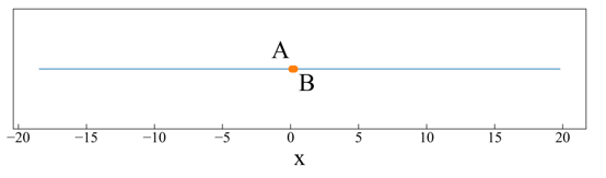
Figure 1: 1D attractor for the Lorenz equation

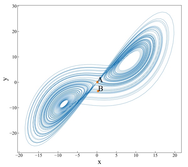
Figure 2: 2D attractor for Lorenz equation

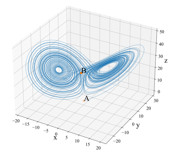
Figure 3: 3D attractor for Lorenz equation

2. FNN Methods

2.1.   Conventional Methods

The authors proposed a method to estimate the minimum embedding dimension in 1992 [5]. Although this approach is simple in principle and works well for many nonlinear systems, it requires an appropriate threshold for every problem. The computational procedure of the FNN method is described in below.

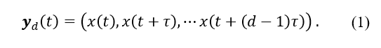
Step 1: Reconstruct the attractor of the time series to be analyzed using Takens’ embedding method [10]. Assuming that the target time series with N samples is x, the lag time is τ, and the embedding dimension is d, the d-dimensional attractor for x is reconstructed by  as follows.

Step 2: Calculate the time  of the nearest neighbor vector of , , according to the distance criterion D.

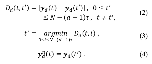
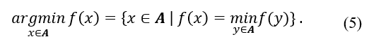
However, the set of x values for which the function  on some set  is minimal is denoted as follows.

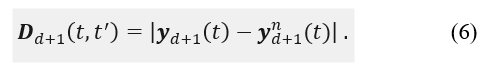
Step 3: Determine the distance  between  and  when the embedding dimension is .

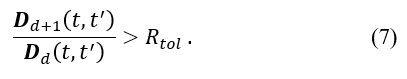
Step 4: Calculate the percentage of vectors in the attractor that are greater than or equal to the given threshold  (false neighbor rate) relative to the rate of change in the neighbor point distance  with increasing embedding dimensions.

Step 5: Repeat the operations in Step 1 to 4 for the given maximum number of embedding dimensions. Then, count from the lowest dimension to the first dimension for which the false neighbor ratio is zero and set the latter as the minimum embedding dimension.

2.2.  Proposed Method

According to this procedure, a neighborhood is considered false when the rate of increase exceeds the threshold value  in Step 4. However, this value must be set for each time series to be analyzed. Therefore, in this study, we propose a false neighborhood reduction rate  as a new criterion to replace the threshold . In Step 4, the rate of increase in the nearest neighbor distance with increasing dimensionality is calculated, and the percentage of vectors the rates of increase of which exceed the threshold value  is calculated. In the proposed approach, the analysis is performed in the same manner up to the point at which the rate of increase of the nearest neighbor distance is obtained, except that the following calculation procedure is used for computable times: .

Step 4’: For the vector  that is the nearest neighbor to the vector  of the attractor at time , find the rate of change of the nearest neighbor distance with increasing embedding dimensions. After applying the ordinary logarithm, the median value is , as given below.

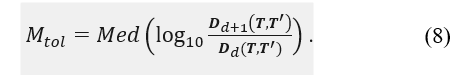
Step 5’: With increasing embedding dimension d, the dimension in which  first becomes less than 1 is considered the minimum embedding dimension, being that in which embedding without false neighbors is established.

Generally, time series may contain noise. Even for time series generated from systems of the same type, noise levels may vary considerably depending on the observation method. For example, consider the case in which the minimum embedding dimension is estimated using the FNN method for a time series with a higher noise level. Owing to the higher noise level, the trajectory of the reconstructed attractor becomes unstable. In this case, the variance of the rate of change of the distance to the nearest neighbor increases with increasing dimensionality. Therefore, the number of points that exceed the given threshold (false nearest neighbors) increases, and the estimated minimum embedding dimension is expected to be high compared to observed time series with less noise. However, because the proposed method refers to the median of the rate of change of the nearest neighbor distance with increasing dimensionality, the effect of increasing variance is expected to be small. Therefore, the proposed approach could serve as a more objective evaluation criterion by eliminating the arbitrariness of the threshold value.

3. Evaluation Method

To compare the FNN method with the proposed method, we used a time series of numerical solutions calculated from a mathematical model in which the variables of the system were known in advance. We considered the van der Pol equation, which depends on two variables, and the Lorenz equation, which depends on three, to investigate whether the estimated embedding dimension was affected by changing the nonlinearity of the time series by setting multiple decay coefficients for the van der Pol equation. In addition, Gaussian noise of 0%, 1%, 10%, and 100% of the standard deviation of the signal was added to the numerical solutions computed from both equations to comprehensively examine their robustness to noise. The minimum embedding dimension was estimated for the time series generated with each parameter setting using both the FNN method and the proposed method, and the difference from the expected minimum embedding dimension was evaluated using the error rate described below.

To demonstrate its applicability to general time series, we applied the proposed approach to time series data recorded from electrooculograms to evaluate how many factors or variables could be identified as underlying nystagmus movements in the system.

3.1.  Van der Pol Equation

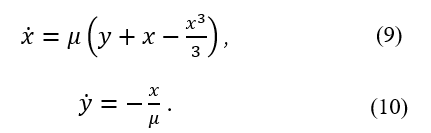
The van der Pol oscillator is among the first examples of deterministic chaos discovered [11]. Van der Pol found a stable oscillation in an electrical circuit using vacuum tubes, which he referred to as the relaxation oscillation. The van der Pol equation is a two-variable differential equation in x and y described by the following equations (9) and (10) with the damping coefficient μ.

In this work, we evaluated whether the numerical solution of the van der Pol equation could be calculated as a second-order system with a minimum embedding dimension for the numerical solution of van der Pol equation. A total of 80 van der Pol time series were generated, including 20 with decay coefficients μ = 0.1, 0.2, … 2.1, and 4 with noise levels of 0%, 1%, 10%, and 100% of the standard deviation of the original time-series signal. For all generated time series, the initial values of x and y were set to 0.1, with a time-step width dt = 0.01, and a time-series length l = 10000 (Figure 4).

3.2.  Lorenz Equation

The Lorenz equation [8] is a nonlinear ordinary differential equation of three variables x, y, and z that exhibits chaotic behavior, as given below. The equations depend on three variables, as shown in the following equations (11), (12), and (13). Lorenz presented this classical equation in 1963 while working on a model of atmospheric variability as a meteorologist at the Massachusetts Institute of Technology [8].

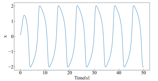
Figure 4: Typical example of van der Pol time series

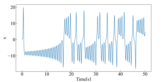
Figure 5: Typical example of Lorenz time series

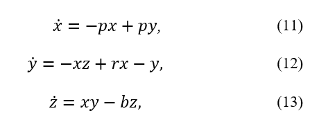
where p, r, and b are constants that determine the behavior of the system.

Numerical solutions of the fourth-order Runge-Kutta method for the Lorenz equation were also obtained for reference, and the displacement x over time was plotted. For the parameter settings p=10, r=28, and b=8/3, the time interval was set to 0.01 second, and the initial values of x, y, and z were set to 0.1.

In this study, the numerical solution of the Lorenz equation was used to evaluate whether it could be calculated as a third-order system with a minimum embedding dimension. To evaluate the Lorenz time series, each parameter value was set to p=10, r=28, b=8/3, and four time series were generated with noise levels of 0%, 1%, 10%, and 100% of the standard deviation. For all generated time series, the initial values of x, y, and z were set to 0.1, the width of the time step dt = 0.01, and length of the time series l = 10000, respectively (Figure 5).

3.3.  Electrooculogram data

An electrooculograms(EOG) is a time series recording changes in the distribution of electric potential around the eye caused by eye movements in two variables x and y. EOG are commonly used to examine the function of the retinal pigment epithelium and analyze eye movements. The electrical characteristics of the data involve a positive potential produced in the cornea closer to the environment and a negative potential produced closer to the retina. During measurement, single electrodes are affixed to a subject’s inner and outer cornea, and their eye movements are recorded electrically via the potential difference between the electrodes [12].

Eye movements are divided into four types, including fixation, in which the eye concentrates on a single spot, pursuit, in which the eye slowly follows an object in the central fossa, saccadic and impulsive movements, in which the eye immediately detects anomalies, and vestibular movements, in which the eye responds to body movements when the body moves. The ocular muscles attached to the eyeballs move the eye and include the lateral rectus, medial rectus, superior rectus, inferior rectus, superior oblique, and inferior oblique muscles, as well as the upper eyelid elevator muscle, which is responsible for eye-opening action. Of the ocular muscles, the lateral rectus muscle is innervated by the abducens nerve, the superior oblique muscle by the pulmonic nerve, and all other muscles by the oculomotor nerve [13–15].

The EOG data used in this study were obtained from 11 healthy subjects (three men and eight women) aged 20-23 years. The subjects viewed experimental 3D images for 180 s each, and the angular velocity of their eye movement during this time was measured [16] (Figure 6).

3.4.  Evaluation: definition of error value

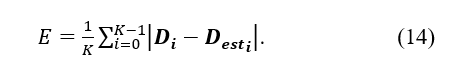
We defined the error value as an index to evaluate the minimum embedding dimension obtained using the FNN algorithm and the proposed method. In this study, we used formula (14), where  is the minimum embedding dimension expected for the time series generated for each parameter setting,  is the minimum embedding dimension estimated from each method for those time series, and K is the total number of parameters when varying the attenuation coefficient and the amount of noise added using the error value E.

4. Results

For Van der Pol Equation and Lorenz Equation, we report the estimated minimum embedding dimension and the error values of the expected minimum embedding dimension and the estimated values from the FNN method and the proposed method. However, for the Van der Pol Equation and Lorenz Equation, multiple time series were prepared under various conditions, so the estimated minimum embedding dimension is reported as an aggregate using the median value for each noise level. For the error between the expected minimum embedding dimension and the estimated value, we also report the error values aggregated by  for the FNN method. The proposed method reports one error value per equation, since there is no threshold such as .

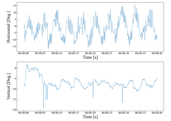
Figure 6: Typical example of an electrooculogram time series

Next, we report the results of estimating the minimum embedding dimension by each method for EOGs as an example of actual observed data.

4.1.  Van der Pol Equation

First, we report on the estimated minimum embedding dimension for each method: the FNN method shows two dimensions when the noise level is 0%. The FNN method shows 2 dimensions when the noise level is 0%, 4 dimensions when the noise level is 1%, 5 dimensions when the noise level is 10%, and 6 dimensions when the noise level is 100%. On the other hand, the proposed method shows two dimensions when the noise level is 0% and 1%, and three dimensions when the noise level is 10% or higher.

Next, we report the error values for the estimated and expected minimum embedding dimension. When  was set in the range of 1, 2, 4, and 1024 in the FNN method, the error value was minimized when =1024. In addition, the proposed method exhibited the same error value as when =1024 (Figure 7).

4.2.  Lorenz Equation

First, we report on the estimated minimum embedding dimension for each method: the FNN method shows 6 dimensions for all noise levels from 0% to 100%, while the proposed method shows 2 dimensions for noise levels of 0% and 1%, and 3 dimensions for noise levels above 10%. On the other hand, the proposed method shows two dimensions for noise levels of 0% and 1%, and three dimensions for noise levels above 10%.

Next, we report the error values for the estimated and expected minimum embedding dimension. When  was set in the range of 1, 2, 4, and 1024 in the FNN method, the error value was the smallest when =512,1024. In the proposed method, the error value was smaller than =256 and larger than =512, 1024 (Figure 8).

4.3.  Electrooculogram data

For the variation in the horizontal axis, the minimum embedding dimensions were estimated using the FNN and proposed methods. With the FNN method,  was estimated to be 1, 2, 4…, 1024. Assuming that the error value of the estimated minimum embedding dimension was smallest when =1024 in 4.1 and that 4.2 and can be applied to EOG data, the horizontal variation of EOG data by the FNN method was estimated and was considered as a system consisting of approximately 4 to 6 variables. In the vertical direction, the same can be considered as a system consisting of 8 to 11 variables. In contrast, using the proposed method, the minimum embedding dimension was estimated as two to three dimensions in the horizontal direction and two dimensions in the vertical direction, suggesting that the system is composed of approximately two to three variables (Figure 9-10).

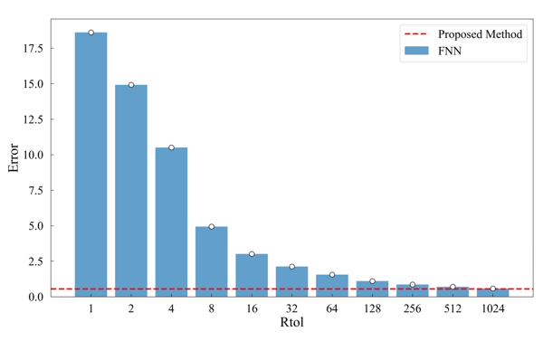
Figure 7: Error rate in estimating the minimum embedding dimension for van der Pol time series using the FNN method and the proposed method

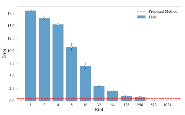
Figure 8: Error rate in estimating the minimum embedding dimension for Lorenz time series using the FNN method and the proposed method

5. Discussion

To compare the FNN method with the proposed approach, we considered a time series of numerical solutions calculated from a mathematical model in which the number of variables constituting the system is known in advance. In this study, the van der Pol equation consisting of two variables and the Lorenz equation consisting of three variables were used, and the difference between the expected minimum embedding dimension and the minimum embedding dimension calculated using each method was evaluated as an error value. First, we discuss the estimation results of the minimum embedding dimension by the proposed method and the FNN method. Next, we discuss the error values between the minimum embedding dimension estimated by each method and the actual minimum embedding dimension. Finally, we discuss the results of estimating the minimum embedding dimension by each method for EOGs as an example of actual observed data.

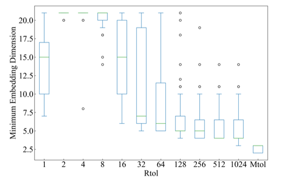
Figure 9: Estimation of the minimum embedding dimension for the horizontal-axis electrooculogram data

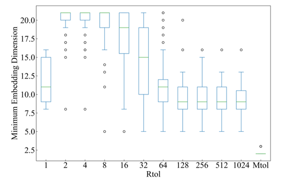
Figure 10: Estimation of the minimum embedding dimension for the vertical-axis electrooculogram data

5.1.  Van der Pol Equation

The estimates of the minimum embedding dimension are discussed: both the FNN method and the proposed method show a minimum embedding dimension of 2 dimensions when the noise level is 0%. This is also the case for the FNN method in [17]. However, the FNN method suggested that the estimate may be vulnerable to noise, since an increase in the noise level to 1% resulted in a three-dimensional estimate. On the other hand, the proposed method did not affect the estimates until the noise level exceeded 10%, suggesting that it may be more robust against noise when compared to the FNN method.

Next, we discuss the error between the estimated first embedding dimension and the expected minimum embedding dimension for each method: the FNN method showed the smallest error when =1024. At this time, the proposed method also showed a comparable error. In other words, the proposed method does not require any threshold adjustment and shows the same error as the optimal value in the FNN method. Of course, since the error tends to decrease as  increases, it is conceivable that the error would decrease more when the threshold is further increased. However, since the decrease in error stalls when  exceeds 256, the decrease in threshold value is considered to be limited even if the threshold value is increased. In addition, it is difficult to determine the optimal value of  because there are situations where the nature and data noise level are unknown in the actual time series to be analyzed. Even if the threshold is set in advance with a large value, it is believed that there may be cases where the minimum embedding dimension is underestimated.

5.2.  Lorenz Equation

The estimates of the minimum embedding dimension are discussed: the FNN method estimated the minimum embedding dimension to be 6 under all noise levels of 0%, 1%, 10%, and 100%. It can be seen that even when the noise level is 0%, the results are very different from what one would expect. To reiterate, this estimate uses the median of the output values estimated for various  settings, so it may output 3, the expected minimum embedding dimension, when the appropriate  is set. Conversely, if an appropriate  cannot be set, it is difficult to estimate the appropriate minimum embedding dimension. On the other hand, the proposed method is considered to be tolerant to noise because it could output the expected minimum embedding dimension even when relatively large noise levels of 10% and 100% were introduced. On the other hand, when the noise levels were relatively low (0% and 1%), the proposed method estimated one dimension less than the expected minimum embedding dimension. This may indicate that the minimum embedding dimension may be underestimated for time series with little disturbance.

Next, we discuss the error between the estimated embedding dimension and the expected minimum embedding dimension for each method: the FNN method showed the smallest error when  = 512 and 1024. In this case, when  is set to a value of 512 or 1024, the optimal minimum embedding dimension can be obtained even after considering the effects of various noises. On the other hand, if  is set to a value higher than 1024, there is a possibility that the minimum embedding dimension will be underestimated. On the other hand, the proposed method had a smaller error value than the FNN method when  was less than 512, but the FNN method had a smaller error value when  was greater than 512. From these results, it can be said that if the optimal  can be set, the FNN method has a smaller error value, i.e., a more accurate estimation of the minimum embedding dimension, but in most cases, the proposed method has a more accurate estimation value.

5.3.  Electrooculogram data

To demonstrate an application to general time series, we applied both the FNN method and the proposed method to EOG data to determine the minimum embedding dimension and examined how many variables the eye movements consist of in the system. The results show that the FNN method found 4 to 6 dimensions in the horizontal direction and 8 to 11 dimensions in the vertical direction. In contrast, the proposed method suggested 2 to 3 dimensions in the direction of the horizontal axis and 2 dimensions in the vertical direction. Several mathematical models of eye movements have been devised, and the Westheimer model s[18–20] is a representative example. In this model, human eye movements are described by a third-order differential equation, which is also close to the minimum embedding dimension calculated by the method proposed in this work.

6. Conclusion

In this study, we have proposed a method to solve the arbitrariness of the threshold used in the FNN method for time series. We have also applied the proposed method to EOG data as an example, and compared the performance of the FNN method and the proposed method in estimating the number of factors that determine eye movements. Compared to the FNN method, the minimum embedding dimension calculated by the proposed method exhibited a lower error value than expected under various conditions. The proposed approach mitigates the difficulty of setting appropriate parameters for a time series of unknown nature and obviates the need for an arbitrary threshold value. In future research, we intend to verify the effectiveness of the proposed method by applying it to a wider range of general time series.

Conflict of Interest

The authors declare no conflict of interest.

1. I.J. Goodfellow, J. Pouget-Abadie, M. Mirza, B. Xu, D. Warde-Farley, S. Ozair, A. Courville, Y. Bengio, “Generative adversarial nets,” in Advances in Neural Information Processing Systems, 2014, doi:10.3156/jsoft.29.5_177_2.
2. A. Radford, L. Metz, S. Chintala, “Unsupervised representation learning with deep convolutional generative adversarial networks,” in 4th International Conference on Learning Representations, ICLR 2016 – Conference Track Proceedings, 2016.
3. F. Kinoshita, Y. Mori, Y. Matsuura, H. Takada, M. Miyao, “A study of numerical analysis and mathematical modeling of electrogastrograms in the young subjects,” IEEJ Transactions on Electronics, Information and Systems, 136(9), 2016, doi:10.1541/ieejeiss.136.1261.
4. Y. Jono, T. Tanimura, F. Kinoshita, H. Takada, “Evaluation of Numerical Solution of Stochastic Differential Equations Describing Body Sway Using Translation Error,” Forma, 35(1), 2020, doi:10.5047/forma.2020.006.
5. M.B. Kennel, R. Brown, H.D.I. Abarbanel, “Determining embedding dimension for phase-space reconstruction using a geometrical construction,” Physical Review A, 45(6), 1992, doi:10.1103/PhysRevA.45.3403.
6. R. Hegger, H. Kantz, “Improved false nearest neighbor method to detect determinism in time series data,” Physical Review E – Statistical Physics, Plasmas, Fluids, and Related Interdisciplinary Topics, 60(4 B), 1999, doi:10.1103/physreve.60.4970.
7. S. Wallot, D. Mønster, “Calculation of Average Mutual Information (AMI) and false-nearest neighbors (FNN) for the estimation of embedding parameters of multidimensional time series in matlab,” Frontiers in Psychology, 9(SEP), 2018, doi:10.3389/fpsyg.2018.01679.
8. E.N. Lorenz, “Deterministic Nonperiodic Flow,” Journal of the Atmospheric Sciences, 20(2), 1963, doi:10.1175/1520-0469(1963)020<0130:dnf>2.0.co;2.
9. J. Milnor, “On the concept of attractor,” Communications in Mathematical Physics, 99(2), 1985, doi:10.1007/BF01212280.
10. F. Takens, Detecting strange attractors in turbulence, 1981, doi:10.1007/bfb0091924.
11. Balth. van der Pol, “ LXXXVIII. On ‘relaxation-oscillations’ ,” The London, Edinburgh, and Dublin Philosophical Magazine and Journal of Science, 2(11), 1926, doi:10.1080/14786442608564127.
12. W.C. Lara, B.L. Jordan, G.M. Hope, W.W. Dawson, R.A. Foster, S. Kaushal, “Fast Oscillations of the Electro-oculogram in Cystic Fibrosis,” Investigative Ophthalmology & Visual Science, 44(13), 4957, 2003.
13. Z.M. Hafed, J.J. Clark, “Microsaccades as an overt measure of covert attention shifts,” Vision Research, 42(22), 2002, doi:10.1016/S0042-6989(02)00263-8.
14. H. Kobayashi, Y. Watanabe, N. Ohashi, K. Mizukoshi, “Pendular Optokinetic Nystagmus Test in Patients with Central Nervous System Disorders,” Practica Otologica, Supplement, 1989, 1989, doi:10.5631/jibirinsuppl1986.1989.Supplement36_133.
15. R. Engbert, R. Kliegl, “Microsaccades uncover the orientation of covert attention,” Vision Research, 43(9), 2003, doi:10.1016/S0042-6989(03)00084-1.
16. A. Sugiura, R. Ono, Y. Itazu, H. Sakakura, H. Takada, “Analysis of Characteristics of Eye Movement While Viewing Movies and Its Application,” Nihon Eiseigaku Zasshi. Japanese Journal of Hygiene, 77, 2022, doi:10.1265/jjh.21004.
17. E. Conte, A. Federici, G. Pierri, L. Mendolicchio, J.P. Zbilut, A brief note on recurrence quantification analysis of bipolar disorder performed by using a van der Pol oscillator model, 2009.
18. G. Westheimer, “Mechanism of saccadic eye movements,” A.M.A. Archives of Ophthalmology, 52(5), 1954, doi:10.1001/archopht.1954.00920050716006.
19. K. Shimono, M. Kondo, K. Shibuta, S. Nakamizo, “Psychophysical and vergence responses of normal and stereoanomalous observers to pulse-disparity stimulus,” The Japanese Journal of Psychology, 53(3), 1982, doi:10.4992/jjpsy.53.136.
20. P.D.S.H. Gunawardane, R.R. Macneil, L. Zhao, J.T. Enns, C.W. de Silva, M. Chiao, “A fusion algorithm for saccade eye movement enhancement with eog and lumped-element models,” IEEE Transactions on Biomedical Engineering, 68(10), 2021, doi:10.1109/TBME.2021.3062256.

(Click Here)