1. Introduction

Energy requirements of a country are met through proper planning, execution, and prediction based on the infrastructure and the availability of resources. It is no surprise that energy consumption has been rising aggressively across the globe with the increasing energy issues, while more attention must be focused on reducing environmental pollution, together with keeping up the economic growth [1,2]. Energy planning for the future is of utmost importance as it can have a significant impact on the economy of a country [3]. Broadly, energy demand has been mainly influenced by the price of energy and earnings, distributional effects, literacy of energy use among society, and the demand for energy in industry and transportation. Particularly the aspects that affect the demand for energy in the country are the climate of the region, urbanization rate [4], the sectorial energy consumption [5], use of technology [6], transition to renewable energy [7], and adherence and enforcement of environmental law and governmental policies [8].

The evolution of the energy sector and the uncertainties related to it have been a topic of interest to strategize energy secure future and layout policies for future energy demand. In this view, recently, a lot of focus has been realized on the modeling tools, frameworks, and assessment procedures that can provide more accurate insight into the future energy demand of a country [9]. Various approaches can be found in the literature dealing with the modeling energy demand in total of a country such as Turkey [10], China and India [11], Spain [12], etc. The recent ones involve the use of metaheuristics for estimating and predicting the energy demand for the future. We now look at various approaches presented in the literature for estimating and predicting country-wide energy demand.

In [11], the authors analyzed the performance of time series forecasting methods (using a grey model) to predict China’s and India’s future energy demand (1990-2016). The reported techniques were deemed to increase the prediction of the future energy demand of the two considered countries. Trend map, error measure, and fit method were used to analyze the accuracy and the mean absolute error of single-linear, hybrid-linear, and non-linear techniques were reported as 1.30-3.08%, 0.80-2.57%, and 2.06-2.19%, respectively. In [12], the authors presented a one-year-ahead estimation of energy demand based on historical data for the years 1980 to 2011 for 14 socio-economic indicators. Modified Harmony Search (HS) and an Extreme Learning Machine (ELM) were used and compared for prediction. Reported results by the proposed approaches made very accurate energy demand predictions with a mean absolute error of 3.21-4.63%. In a similar work [13], the authors analyzed the performance of the robust hybrid approach composed of a Basic Variable Neighbourhood Search (BVNS) algorithm with ELM. BVNS was employed to select the most suitable macroeconomic features from the large group of considered ones, whereas the ELM performed the energy demand predictions on the considered features. The proposed algorithm was reported to have the best Mean absolute  error lower than 1.66% and an average Mean absolute error of 3.90%. In [14], the authors proposed a new framework for energy demand estimation by combining an adaptive Genetic Algorithm (GA) and a co-integration analysis for China. Model weights were optimized using Artificial Intelligence techniques (GA, ACO, and hybrid algorithms) together with co-integration analysis. It was reported that the proposed models have significantly better performance (Mean Absolute Percentage Error, of 8.68%). In [15], the authors proposed a hybrid algorithm formed by Bat Algorithm, Gaussian Perturbations, and Simulated Annealing Energy Demand (BAG-SA EDE) for China data. The analysis of the relationship between the energy demand and the input factors was carried out using a stationary test, co-integration test, and Granger causality test. It was reported that the quadratic model performs better prediction (mean absolute percentage error of 0.28%) of future energy demand than the multiple linear regression (mean absolute percentage error of 0.88%). Grammatical Evolution (GE) was proposed by [16] for developing new models using 14 macro-economic parameters for a year-ahead estimation of country-wide energy demand for Spain and France. The Differential Evolution (DE) algorithm was used to optimize each model’s parameters. The proposed algorithms exhibited excellent accuracy (best Mean absolute error 1.9, and average Mean absolute error 3.33) for energy prediction. Bees Algorithm technique was suggested in [17] for estimating total energy demand in Iran based on population, GDP, import, and export data. Exponential and linear models were proposed for estimation and were also deployed to predict energy demand for up to the year 2030. It was concluded that the linear Bees Algorithm technique has the best prediction accuracy (relative error of 1.07%). In [18], the authors demonstrated a Mix-encoding Particle Swarm Optimization and Radial Basis Function (MPSO-RBF) based energy demand forecasting for China until the year 2020.  The input data (for the years 1980-2009) consists of GDP, population, industry proportion, urbanization rate, and share of coal energy. It was reported that the proposed MPSO-RBF has four nodes of hidden layers and better accuracy in terms of the errors (Mean absolute  percentage error of 0.78%) when compared to other Artificial Neural Networks (ANN)[19] based models. In [20], Particle Swarm Optimization and Genetic Algorithm optimal Energy Demand Estimating (PSO-GAEDE) model was proposed to improve the estimation efficiency for future projection in China. Linear, quadratic and exponential forms of models were proposed based on historical data from 1990 to 2009. The proposed PSO-GAEDE algorithm was reported to perform better than other algorithms with a Mean absolute percentage error of 0.54%. In [21], the authors deployed an ANN (with feed-forward multilayer perceptron model, coupled with an error back-propagation technique, FF-BP-ANN) to estimate the energy demand for Korea. Multiple linear regression models, exponential model, and ANN models [22] were analyzed and it was concluded that the ANN model outperforms the multiple linear regression models (linear and exponential) with accuracy in terms of Root Mean Squared Error, RMSE=5.7803. In [23], the authors forecasted the energy demand of China using a hierarchical Bayesian approach. Static and dynamic models were proposed with variable input parameters and forecasts were made for years up to 2030. It was reported that the hierarchical Bayesian approach has better performance (RMSE = 0.025) in model fitting than the fixed effects method (RMSE = 0.030). An analysis of energy structure and carbon emissions for China was performed in [24] using an optimized mixed data sampling model (ADL-MIDAS) model involving quarterly GDP, quarterly added value, and annual energy demand as the input variables. It was reported that compared to previous studies, the prediction error (RMSE) was in general below 0.1%, and the smallest error was reported to be 0.02%, thereby energy demand prediction was significantly improved. The forecast of energy demand for the Hunan province of China was presented in [25] between the years 2012 to 2030. Autoregressive integrated moving average and vector autoregressive models were employed for forecasting, and the resulting uncertainties analyzed using the Monte-Carlo method were reported to be under 15%. In [26], the authors employed a swarm intelligence-based Adaptive Firefly Algorithm (AFA) to improve the energy demand estimation in Turkey based on economic parameters.  Linear and quadratic forms of models were proposed for estimation and historical data for Turkey. The proposed models were compared with Ant Colony Optimization (ACO) and Particle Swarm Optimization (PSO), each involving linear and quadratic models. It was concluded that the AFA-quadratic model resulted in the best accuracy with an accuracy of 99.24%. The determinants for energy demand in Turkey were discussed in [27]. ACO was used to optimize the energy demand problem. Three scenarios of energy demand growth were discussed and values of energy demand were determined for Turkey for 2006-2025. The quadratic equation optimized by ACO was suggested to be the most accurate with a deviation of 2.83%. Similar works were also reported by [28]  and [29] for Turkey. Other authors used Differential Evolution (DE)[10], Artificial Algae Algorithm (AAA)[30], PSO [31], Ridge Regression (RR), and Partial Least Squares Regression (PLSR)[32] for estimating future energy demand in Turkey.

Based on previous research, it is elucidated that the long-term dependence of energy demand on economic growth factors certainly exists [33].

In this paper, a one-year-ahead energy demand prediction for Turkey is proposed involving a combination of evolutionary metaheuristic algorithms. These algorithms are based on Grammatical Evolution (GE) and Differential Evolution (DE), where GE has the capacity to develop flexible model forms based on the information provided in the grammar, while DE optimizes the model’s parameters. Utilizing these two algorithms in combination results in better estimation accuracy and the predictions for energy demand can be made with greater reliability. The input variables selected are similar to the previous studies so that the comparison of algorithms is fair and the advantage of the present approach can be highlighted. These variables consist of the historical data of socio-economic parameters: GDP, population, import, and export quantities, which were used as inputs, while Energy demand was the target or output variable.

The novelty of the work is further justified by the comparison of algorithms and the grammars used. In the current scenario, two particular approaches have been proposed: Grammatical Evolution alone, and an ensemble of Grammatical Evolution with Differential evolution. Based on these algorithms, four different proposals were studied:

1. M1: Grammatical Evolution with a recursive grammar.
2. M2: Ensemble of Grammatical Evolution with linear grammar and Differential Evolution.

• M3: Ensemble of Grammatical Evolution with quadratic grammar and Differential Evolution.

1. M4: Grammatical Evolution with a recursive grammar and Differential Evolution.

The performance of these proposals is compared by assessing their estimation accuracy using RMSE as the objective function. The average error, R², absolute error, and relative error metrics were calculated to compare the performance of the proposals.

The present algorithm combination is also compared to the previous research works reported in literature involving Differential Evolution to validate their accuracy.  Further, the application of these metaheuristics is utilized to predict the future energy demand for Turkey. One year ahead energy demand prediction is made using the combination of the previously described two algorithms (GE and DE). Thus, the approach with the combination of the Grammatical Evolution algorithm provided with a highly recursive grammar unified with the optimization strength of the Differential Evolution algorithm (M4) presents a unique and highly accurate approach to making energy demand predictions.

The rest of the paper is organized as follows. Section 2 provides the outline of the methodology used consisting of the data obtained, problem definition, and the objective function. Section 3 discusses the results obtained dealing with the estimation of energy demand and prediction of the year ahead of future energy demand for Turkey. Finally, Section 4 presents the conclusions of the study.

2. Research Methodology and Algorithms

In this section, the proposed methodology is described. Firstly, the used dataset is described as well as the curation, training, and test selection processes. Then, the algorithmic proposals and quality metrics are detailed.

2.1.  Data

The required data for the study consisted of the historical energy demand as well as the corresponding data for socio-economic parameters for Turkey, obtained from literature [10]. This data was compiled from MENR, the energy reports, and some of the previously reported studies in the literature [32]. The data consisted of Turkey’s GDP ($10⁹), Population (10⁶), and the amounts of Import ($10⁹) and Export ($10⁹) for the period from 1979 to 2011 (as annual values). These four elements are generally considered to have the biggest impact on the energy demand. Therefore these are considered as the input variables for the present study as well. The target variable for estimation (as well as prediction), is the energy demand (MTOE). Data obtained can be found in the appendix (Table A.1). Notice that the input variables are also named X1 (GDP), X2 (Population), X3 (Quantity of Imports) to X4 (Quantity of Exports) while the energy demand is denoted as E.

From the historical dataset of the energy demand for Turkey, an interesting trend can be deduced for the period studied.  The energy demand growth rate ranges from a minimum of -6.34% (for the year 2001) to a maximum of 10.38% (for the year 1987) with an average growth rate of 4.26%. While the input parameters growth rate are: GDP (Average 8.41%, minimum -27.00% and maximum 39.81%), population (Average 1.57, minimum -3.26 and maximum 2.95), import (Average 14.81%, minimum -30.22% and maximum 56.02%), and export quantities (Average 14.58%, minimum -22.64% and maximum 61.51%). It will be, therefore, interesting to find out how these socio-economic parameters correlate to energy demand and further their impact on its future.

In order to avoid the influence on a model of the particular amount of each variable (due to the units used in each one of them), all the data have been normalized by the maximum value of each corresponding parameter. This way, every column has been transformed into the values that correspond to the ratio with the maximum value of the data:

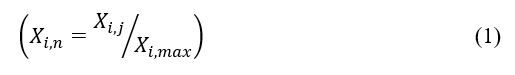
where i = 1, 2, 3, 4. j = 1, 2…n, n being the number of years, and max being the maximum value of the i^th series.

Therefore, the maximum value of a given column is 1, while the rest of the values will be lower. This normalization is also done for the output variable. The data which spans 33 years were divided into two datasets i.e., training and test, where the training dataset consists of data for 17 years and the test dataset consists of the dataset for the remaining 16 years. The selection for each dataset was made randomly.

2.2.  Problem definition and objective function

The search for a mathematical expression that captures the behavior of a target variable can be tackled as an optimization problem. In particular, this approach aims to find the expression with the minimum error, which in this case, is modeling the energy demand.

To assess the quality of a model, the root mean squared error (RMSE) metric, as shown in Equation (2), is used as the objective function.

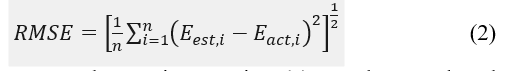
where,  and  in Equation (2) are the actual and estimated values of energy demand.

While other statistics viz, average error (AE), coefficient of determination (R²), absolute error (ABS), and relative error (RE) were also used to evaluate the accuracy as follows:

2.3.  Algorithmic Methods

In this work, the deployment of Grammatical Evolution (GE) and Differential Evolution (DE) is proposed for the estimation of energy demand. GE is a metaheuristic algorithm belonging to the family of Genetic Programming whose main advantage is the ability to direct the search of the algorithm using grammar [34]. This way, researchers may introduce knowledge about the problem into the grammar, reducing the search space. On the other hand, DE is a metaheuristic algorithm better suited for problems where some parameter values need to be found [35].

Despite the combination of GE and DE has been proven to be effective in the past for this problem [16],[36,37], one of the main contributions of this work is the comparison with different combinations of GE and DE determined by different grammars using a reduced number of input variables. The tool used in this work is WebGE, which is an open-source optimization tool that implements both GE and DE algorithms described before. We refer the reader to [38] for further information.

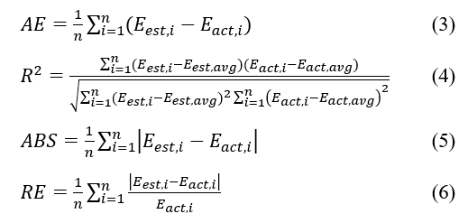
In particular, four different approaches are proposed in this work. The first one is the use of recursive grammar in GE with no DE intervention (M1). Figure 1 shows the grammar applied to this approach. Elements on the left-hand side of each “::=” symbol are non-terminal values, which must be decoded using any of the productions on the right-hand side, separated by “|” symbols. As seen in the figure, this grammar can generate mathematical expressions using the four input variables (X1 to X4), constant values, addition, subtraction, and product arithmetic operators, and the exponential, power, and logarithmic functions. It is important to note that the <param> non-terminal symbol is devoted to generating constant numbers in the range [0.00,99.99].

The second approach, named M2, is directed by the grammar shown in Figure 2. The main idea is to produce expressions where arithmetic combinations of a parameter multiplied by an input variable are generated. In this case, DE is in charge of finding out the best parameter values (w_i) for each expression generated by GE. Notice that the <digit> rule is not needed since the parameters, represented by wi, are found by DE.

The third approach is similar to the previous one but includes the use of the quadratic values of input variables. This approach is termed M3 and is guided by the grammar shown in Figure 3. Again, DE is in charge of finding out the values of the parameters.

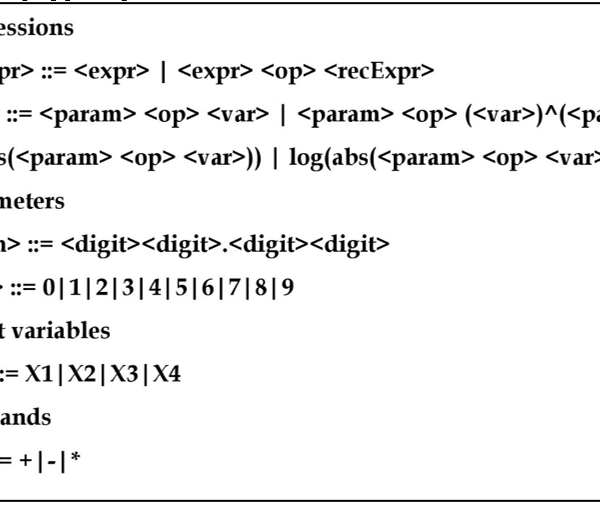
Figure 1: GE executed on a recursive grammar (M1)

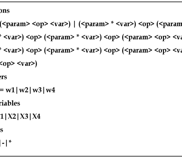
Figure 2: Ensemble of GE executed on a linear grammar and DE (M2)

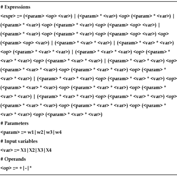
Figure 3: Ensemble of GE executed on quadratic grammar and DE (M3)

Finally, the last approach is the ensemble of GE and DE using recursive grammar. In this case, first, the GE approach is taken, but allowing DE to look for the parameter values. Figure 4 shows the proposed grammar for this approach.

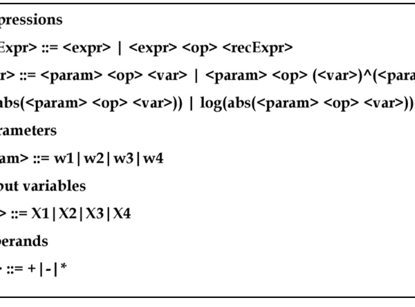
Figure 4: Ensemble of GE executed a recursive grammar and DE (M4)

3. Results and discussion

The experimental experience consisted of the execution of the proposed algorithms over the training dataset under the four configurations presented in the previous section. In particular, 20 runs were executed for each one of the four approaches over the training dataset, obtaining a total amount of 80 different models. Table 1 shows the values of the parameters for the GE and DE algorithms, selected after preliminary experimentation.

Table 1: Details of the experiments

GE Parameters
Generations	50
Crossover Probability	0.65
Population	20
Mutation Probability	0.1
Max wraps	3
Number of Codons	100
Tournament	2
Number of Runs	20
DE Parameters
Recombination Factor	0.88
Mutation Factor	0.47
Population Size	20

 The results presented in the following sections first describe the estimation followed by the prediction. On one hand, for the estimation problem, the values of the input variables of a given year are used to estimate the energy demand of the same year. On the other hand for prediction, the models have been adapted for the prediction of future energy demand, where the values of the input variables of a given year are used to predict the energy demand of the following year.

3.1.  Estimation of Energy Demand

The energy demand estimations were obtained for all the years from 1979 to 2011 using the models generated by the proposed algorithms. In particular, for each one of the four approaches developed under the present study (M1, M2, M3, and M4), an average estimation using the 20 generated models has been evaluated for the target period.

The results of the estimation for the whole dataset are presented in Table 2 considering the average prediction of the 20 models obtained for each one of the four proposed approaches. The previously reported [10] two models Linear (DEL) and Quadratic (DEQ) are also included in this comparison.

Table 2: Estimations of the previously reported differential algorithms based on linear and quadratic [10] with the four model forms of the present approach i.e., M1, M2, M3 and M4

Year	Actual Energy (MTOE)	Linear (DEL) [10]	Quadratic (DEQ) [10]	M1	M2	M3	M4
1979	30.71	32.28	34.48	32.07	30.06	31.88	32.11
1980	31.97	30.89	31.26	29.79	30.71	30.99	31.11
1981	32.05	32.52	33.33	32.09	32.99	32.54	32.67
1982	34.39	34.15	34.84	34.50	34.48	34.01	34.12
1983	35.7	36.53	35.85	36.95	36.29	36.24	36.28
1984	37.43	38.73	37.01	39.50	38.84	38.39	38.39
1985	39.4	40.95	40.10	42.11	40.89	40.43	40.45
1986	42.47	43.27	42.78	44.48	42.27	42.50	42.52
1987	46.88	45.30	45.28	46.89	45.47	44.60	44.63
1988	47.91	46.89	47.68	49.38	47.12	46.02	46.09
1989	50.71	49.76	50.43	51.91	49.40	48.75	48.82
1990	52.98	54.02	53.08	54.55	53.86	53.22	53.25
1991	54.27	55.33	54.49	56.95	54.77	54.25	54.34
1992	56.68	57.52	56.42	59.30	56.85	56.41	56.49
1993	60.26	61.79	61.00	61.71	60.53	61.00	60.92
1994	59.12	60.08	60.48	64.20	59.63	58.79	58.87
1995	63.68	65.28	65.29	66.76	65.26	64.80	64.70
1996	69.86	69.71	70.00	69.41	68.90	69.69	69.41
1997	73.78	72.31	73.17	72.13	71.64	72.54	72.24
1998	74.71	73.30	74.92	74.95	72.50	73.05	72.92
1999	76.77	74.18	75.47	78.44	72.74	73.30	73.29
2000	80.5	80.71	81.04	80.89	77.40	80.84	80.43
2001	75.4	75.71	74.60	83.28	75.13	74.81	74.78
2002	78.33	79.13	80.32	85.65	79.05	78.89	78.86
2003	83.84	82.36	84.01	88.05	84.57	83.47	83.54
2004	87.82	87.19	88.04	90.45	91.57	90.62	90.68
2005	91.58	93.10	92.84	95.31	97.36	97.83	97.90
2006	99.59	96.25	56.00	95.31	101.70	102.69	102.57
2007	107.63	92.76	4.97	88.98	103.98	102.43	102.66
2008	106.27	94.19	-136.98	90.40	109.84	106.49	107.15
2009	106.14	90.17	-495.07	96.02	103.81	96.02	95.47
2010	109.27	103.09	-2.75	99.43	110.96	113.23	113.12
2011	114.48	114.50	64.97	100.12	118.99	129.30	128.27

Highlighted values represent the period of consideration in the study conducted by Beskirli et a [10]

Notice that the previous comparison of algorithms presented in the state of the art was made for a small range of years, corresponding to the period from 1996 to 2005 as highlighted in Table 2. However, in this work, the comparison is made for the entire range of the years (1979-2011) as previously described. Correspondingly, Table 3 compares the estimation performance over the test dataset of the four proposed approaches with the two methods found in the state of the art: a linear model (DEL) and a quadratic model (DEQ). For all of them, 5 error metrics have been obtained: root mean squared error (RMSE), Average Error (AE), R², Absolute Error (ABS), and Relative Error (RE). Notice that the depicted values correspond to the average value of the 20 models in the case of the four proposed approaches.

Table 3: Error metrics for the compared models over the test data. Best results are depicted in bold fonts.

Year	Linear (DEL) [10]	Quadratic (DEQ) [10]	M1	M2	M3	M4
RMSE	4.6403	116.5278	6.1913	3.7255	3.6481	2.2002
AE	2.4685	35.5655	4.0700	2.0997	2.1008	1.6850
R2	0.9771	0.9812	0.9504	0.9807	0.9812	0.9931
ABS	81.4605	1173.6609	134.1800	69.2909	69.3275	55.6063
RE	0.0316	0.3408	0.0520	0.0269	0.0270	0.0238

As seen in the table, all the proposed approaches except M1 (GE with no DE) obtain superior results than the algorithms from the state of the art in terms of the error metrics. Further as observed, the M4 proposal exhibits the top performance among the proposed algorithms with the lowest values of RMSE (2.2002), Average Error (1.6850), Absolute Error (55.6063), Relative Error (0.0238), and the highest value of R² (0.9931). This can be attributed to the fact that the flexible model structure of the recursive grammar combined with the DE efficiency can obtain better parameter values, resulting in a much better performance in comparison to those approaches where the model structure is fixed. Therefore, the ensemble of GE and DE with a recursive grammar (M4) is the most appropriate algorithm for the estimation of energy demand. Hence, this appropriate combination of metaheuristic algorithms (M4) will be used to predict the energy demand for the future.

3.2.  Prediction of Future Energy Demand

The confirmation of the performance improvement achieved from the proposed methods has been made in the previous section. It is established that Model M4 which represents an ensemble of a recursive GE combined with DE has the most accurate outcomes when applied to energy demand problems.

We now move on to the problem of predicting the year-ahead energy demand. To this aim, the set of input parameters remains the same as they were previously discussed. However, the algorithm took the previous year’s data as input variables to predict the energy demand for the current year. This way a year ahead energy demand approach is established. In a similar fashion, the training and test datasets were separated, where the training dataset was used to train the algorithms while the test dataset was used as independent data to test the performance of the algorithms.

The experimentation then followed the same pattern: 20 runs were executed for the GE with a recursive grammar together with DE combination (with the same properties as previously discussed in Table 1) over the training dataset which produced the 20 models (which can be found in Appendix Table A.2). The results of the performance of algorithms in predicting the future energy demand are depicted in figures 5 (a) and (b) for training and test dataset, respectively, as an average of the 20 runs executed for energy prediction. It must be again noted here that since the input to the algorithm is normalized the output that is received is also in the normalized form. This can also be observed in figures 5(a) and (b).

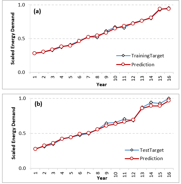
Figure 5: Predicted and actual energy demand (normalized) on (a) training and (b) test datasets. The X-axis denotes the ordinal number of the year in the dataset.

From the figure, it is observed that the predictions match the data very precisely and the errors are small. Table 4 shows the error metrics obtained for the prediction of a year ahead energy demand with M4. It is observed that the algorithm has high accuracy and performs well in terms of prediction accuracy as justified by the small errors produced on the test dataset. Also, since the training and test datasets were independent the issue of overfitting a model on the data is avoided, resulting in a more flexible and accurate model. The predictions of energy demand are presented below in Figure 6 with actual MTOE units for the complete dataset. As seen, the proposed method shows high accuracy on a one-year ahead prediction.

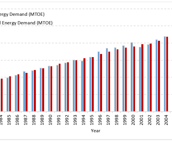
Figure 6: Evolution and comparison of actual and predicted energy demand (using the average of the 20 experimental runs)

The error computation is also made based on Figure. 6 and the obtained results were the following: RMSE=2.2278, AE=-0.6099, R²= 0.9970, ABS=1.7263, and RE =0.0244. As seen, they are similar to the results with separated training and test data.

Table 4: Errors between predicted values from M4 and actual data for energy demand (normalized)

Error	Training	Test
RMSE	0.0146	0.0233
AE	0.0001	0.0107
R2	0.9952	0.9959
ABS	0.1917	0.2908
RE	0.0210	0.0279

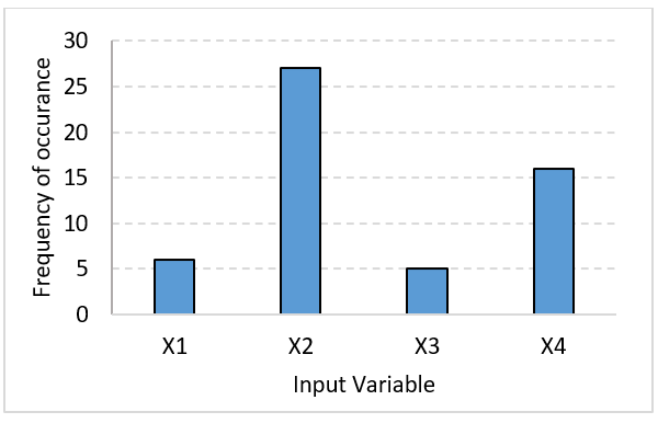
Figure 7: Histogram obtained from 20 runs of GE-DE

The details of prediction models are provided in the appendix (Table A.2). On further analysis of the obtained models, the number of terms appearing in the expressions ranges from 2 to 5, where some of the input parameters appear several times in the different model as well as different expressions. This leads us to find out the most influential parameter among the set of input parameters. To this aim, we calculate the frequency of occurrence of the four input parameters in the 20 models. The occurrence of the feature or the input variable in the equations is depicted in Figure 7. It can be observed that X2 (Population) appears the maximum number of times in the equations, followed by the X4 (quantity of export), the input X1 (GDP), and lastly the X3 (quantity of import). This means that energy demand primarily grows in correlation to the population of the country which in fact is imperative since the larger the population, the more is energy demand.

4. Conclusions

Country-wide energy demand predictions have been made considering socio-economic parameters based on metaheuristic algorithms for Turkey. Four methods were considered initially for the estimation of energy demand: (M1) Grammatical Evolution with a recursive grammar alone, (M2) Grammatical Evolution with a linear grammar together with Differential Evolution, (M3) Grammatical Evolution with a quadratic grammar together with Differential Evolution, and finally, (M4) Grammatical Evolution with a recursive grammar combined with Differential Evolution. The ensemble of GE with a recursive grammar and DE together (M4) performed very well in comparison to others with the least value of objective function RMSE=2.2002. Further, this M4 proposal was deployed to predict a year-ahead energy demand for Turkey. The algorithm again performed very well obtaining the predictions for a year ahead, and the results of prediction were deemed to be exceptionally well with the objective function to be RMSE=2.2278. Therefore, it is recommended to use the combination of Grammatical Evolution with recursive grammar to provide for more flexible model forms. Further, the use of Differential Evolution together with the recursive algorithm of GE provides optimization of the model weight leading to accurate predictions of the energy demand for a country. It was also inferred that population greatly affects the structure of the prediction models and thus is a significant parameter for energy demand models. It is suggested that for future studies long-term causal relationships are established along with the elasticities of algorithms. This will be significant and reflect a more certain behavior to predict the energy demand. Further, it is advised to investigate the behavior of algorithms with more input parameters to elucidate influential and non-influential parameters for energy demand estimation/prediction. This can also implicate the direct and indirect relationship between the input parameters and the energy demand.

Conflict of Interest

The authors declare no conflict of interest.

Acknowledgment

The work reported under the manuscript has received funding from the European Union’s Horizon 2020 research and innovation programme under the Marie Skłodowska-Curie grant agreement No. 754382. The authors would like to thank Prof. Abraham Duarte for extending his support towards the research work carried out in the article.

1. S. Katircioglu, C. Köksal, S. Katircioglu, “The role of financial systems in energy demand: A comparison of developed and developing countries,” Heliyon, 7(6), e07323, 2021, doi:https://doi.org/10.1016/j.heliyon.2021.e07323.
2. S. Di Leo, P. Caramuta, P. Curci, C. Cosmi, “Regression analysis for energy demand projection: An application to TIMES-Basilicata and TIMES-Italy energy models,” Energy, 196, 117058, 2020, doi:https://doi.org/10.1016/j.energy.2020.117058.
3. C. Huang, Z. Zhang, N. Li, Y. Liu, X. Chen, F. Liu, “Estimating economic impacts from future energy demand changes due to climate change and economic development in China,” Journal of Cleaner Production, 311, 127576, 2021, doi:https://doi.org/10.1016/j.jclepro.2021.127576.
4. Y. Yu, N. Zhang, J.D. Kim, “Impact of urbanization on energy demand: An empirical study of the Yangtze River Economic Belt in China,” Energy Policy, 139, 111354, 2020, doi:https://doi.org/10.1016/j.enpol.2020.111354.
5. S. Qiu, T. Lei, J. Wu, S. Bi, “Energy demand and supply planning of China through 2060,” Energy, 234, 121193, 2021, doi:https://doi.org/10.1016/j.energy.2021.121193.
6. J. Huang, H. Zhang, W. Peng, C. Hu, “Impact of energy technology and structural change on energy demand in China,” Science of The Total Environment, 760, 143345, 2021, doi:https://doi.org/10.1016/j.scitotenv.2020.143345.
7. K. Oshiro, S. Fujimori, Y. Ochi, T. Ehara, “Enabling energy system transition toward decarbonization in Japan through energy service demand reduction,” Energy, 227, 120464, 2021, doi:https://doi.org/10.1016/j.energy.2021.120464.
8. P. Späth, H. Rohracher, “Local Demonstrations for Global Transitions—Dynamics across Governance Levels Fostering Socio-Technical Regime Change Towards Sustainability,” European Planning Studies, 20(3), 461–479, 2012, doi:10.1080/09654313.2012.651800.
9. M.A. Islam, H.S. Che, M. Hasanuzzaman, N.A. Rahim, Chapter 5 – Energy demand forecasting, Academic Press: 105–123, 2020, doi:https://doi.org/10.1016/B978-0-12-814645-3.00005-5.
10. M. BESKIRLI, H. HAKLI, H. KODAZ, “The energy demand estimation for Turkey using differential evolution algorithm,” Sādhanā, 42(10), 1705–1715, 2017, doi:10.1007/s12046-017-0724-7.
11. Q. Wang, S. Li, R. Li, “Forecasting energy demand in China and India: Using single-linear, hybrid-linear, and non-linear time series forecast techniques,” Energy, 161, 821–831, 2018, doi:https://doi.org/10.1016/j.energy.2018.07.168.
12. S. Salcedo-Sanz, J. Muñoz-Bulnes, J.A. Portilla-Figueras, J. Del Ser, “One-year-ahead energy demand estimation from macroeconomic variables using computational intelligence algorithms,” Energy Conversion and Management, 99, 62–71, 2015, doi:https://doi.org/10.1016/j.enconman.2015.03.109.
13. J. Sánchez-Oro, A. Duarte, S. Salcedo-Sanz, “Robust total energy demand estimation with a hybrid Variable Neighborhood Search – Extreme Learning Machine algorithm,” Energy Conversion and Management, 123, 445–452, 2016, doi:https://doi.org/10.1016/j.enconman.2016.06.050.
14. J. Huang, Y. Tang, S. Chen, “Energy Demand Forecasting: Combining Cointegration Analysis and Artificial Intelligence Algorithm,” Mathematical Problems in Engineering, 2018(5194810), 1–13, 2018, doi:10.1155/2018/5194810.
15. Q. Wu, C. Peng, “A hybrid BAG-SA optimal approach to estimate energy demand of China,” Energy, 120, 985–995, 2017, doi:https://doi.org/10.1016/j.energy.2016.12.002.
16. J.M. Colmenar, J.I. Hidalgo, S. Salcedo-Sanz, “Automatic generation of models for energy demand estimation using Grammatical Evolution,” Energy, 164, 183–193, 2018, doi:https://doi.org/10.1016/j.energy.2018.08.199.
17. M.A. Behrang, E. Assareh, M.R. Assari, A. Ghanbarzadeh, “Total Energy Demand Estimation in Iran Using Bees Algorithm,” Energy Sources, Part B: Economics, Planning, and Policy, 6(3), 294–303, 2011, doi:10.1080/15567240903502594.
18. S. Yu, Y.-M. Wei, K. Wang, “China’s primary energy demands in 2020: Predictions from an MPSO–RBF estimation model,” Energy Conversion and Management, 61, 59–66, 2012, doi:https://doi.org/10.1016/j.enconman.2012.03.016.
19. X. Yin, Q. Zhang, H. Wang, Z. Ding, “RBFNN-Based Minimum Entropy Filtering for a Class of Stochastic Nonlinear Systems,” IEEE Transactions on Automatic Control, 65(1), 376–381, 2020, doi:10.1109/TAC.2019.2914257.
20. S. Yu, Y.-M. Wei, K. Wang, “A PSO–GA optimal model to estimate primary energy demand of China,” Energy Policy, 42, 329–340, 2012, doi:https://doi.org/10.1016/j.enpol.2011.11.090.
21. Z.W. Geem, W.E. Roper, “Energy demand estimation of South Korea using artificial neural network,” Energy Policy, 37(10), 4049–4054, 2009, doi:https://doi.org/10.1016/j.enpol.2009.04.049.
22. J. Liu, Y. Liu, Q. Zhang, “A weight initialization method based on neural network with asymmetric activation function,” Neurocomputing, 483, 171–182, 2022, doi:https://doi.org/10.1016/j.neucom.2022.01.088.
23. X.-C. Yuan, X. Sun, W. Zhao, Z. Mi, B. Wang, Y.-M. Wei, “Forecasting China’s regional energy demand by 2030: A Bayesian approach,” Resources, Conservation and Recycling, 127, 85–95, 2017, doi:https://doi.org/10.1016/j.resconrec.2017.08.016.
24. Y. He, B. Lin, “Forecasting China’s total energy demand and its structure using ADL-MIDAS model,” Energy, 151, 420–429, 2018, doi:https://doi.org/10.1016/j.energy.2018.03.067.
25. R. Chen, Z. Rao, G. Liu, Y. Chen, S. Liao, “The long-term forecast of energy demand and uncertainty evaluation with limited data for energy-imported cities in China: a case study in Hunan,” Energy Procedia, 160, 396–403, 2019, doi:https://doi.org/10.1016/j.egypro.2019.02.173.
26. H. Wang, Z. Chen, W. Wang, Z. Wu, K. Wu, W. Li, “Improving Energy Demand Estimation Using an Adaptive Firefly Algorithm BT – Computational Intelligence and Intelligent Systems,” in: Li, K., Li, W., Chen, Z., and Liu, Y., eds., Springer Singapore, Singapore: 171–181, 2018.
27. M. Duran Toksarı, “Ant colony optimization approach to estimate energy demand of Turkey,” Energy Policy, 35(8), 3984–3990, 2007, doi:https://doi.org/10.1016/j.enpol.2007.01.028.
28. A. Ünler, “Improvement of energy demand forecasts using swarm intelligence: The case of Turkey with projections to 2025,” Energy Policy, 36(6), 1937–1944, 2008, doi:https://doi.org/10.1016/j.enpol.2008.02.018.
29. O. ERSEL CANYURT, H. CEYLAN, H. KEMAL OZTURK, A. HEPBASLI, “Energy Demand Estimation Based on Two-Different Genetic Algorithm Approaches,” Energy Sources, 26(14), 1313–1320, 2004, doi:10.1080/00908310490441610.
30. A. Beşkirli, M. Beşkirli, H. Haklı, H. Uğuz, “Comparing Energy Demand Estimation Using Artificial Algae Algorithm : The Case of Turkey,” Journal of Clean Energy Technologies, 6(4), 349–352, 2018, doi:10.18178/jocet.2018.6.4.487.
31. T. Paksoy, G. Weber, “Particle Swarm Optimization Approach for Estimation of Energy Demand of Turkey,” Global Journal of Technology & Optimization, 3(June), 1–9, 2012.
32. Y.M. Bulut, Z. Yildiz, “Comparing energy demand estimation using various statistical methods: The case of Turkey,” Gazi University Journal of Science, 29(2), 237–244, 2016.
33. A. Löschel, S. Managi, “Recent Advances in Energy Demand Analysis—Insights for Industry and Households,” Resource and Energy Economics, 56, 1–5, 2019, doi:https://doi.org/10.1016/j.reseneeco.2019.04.001.
34. M. O’Neill, C. Ryan, “Grammatical evolution,” IEEE Transactions on Evolutionary Computation, 5(4), 349–358, 2001, doi:10.1109/4235.942529.
35. R. Storn, K. Price, “Differential Evolution – A Simple and Efficient Heuristic for global Optimization over Continuous Spaces,” Journal of Global Optimization, 11(4), 341–359, 1997, doi:10.1023/A:1008202821328.
36. N. Lourenço, J.M. Colmenar, J.I. Hidalgo, S. Salcedo-Sanz, “Evolving energy demand estimation models over macroeconomic indicators,” GECCO 2020 – Proceedings of the 2020 Genetic and Evolutionary Computation Conference, 1143–1149, 2020, doi:10.1145/3377930.3390153.
37. B. Jamil, L. Serrano-Luján, J.M. Colmenar, “Modelling energy consumption in Spain with metaheuristic methods,” in 2021 6th International Conference on Smart and Sustainable Technologies (SpliTech), 1–3, 2021, doi:10.23919/SpliTech52315.2021.9566391.
38. J.M. Colmenar, R. Martín-Santamaría, J.I. Hidalgo, “WebGE: An Open-Source Tool for Symbolic Regression Using Grammatical Evolution BT – Applications of Evolutionary Computation,” in: Jiménez Laredo, J. L., Hidalgo, J. I., and Babaagba, K. O., eds., Springer International Publishing, Cham: 269–282, 2022.

(Click Here)