1. Introduction

This paper is an extension of the work originally presented in ICITEE 2021 with 1) addition of classification problems and 2) more clarified outcomes (i.e. graphs, tables) [1].

ML models are widely used in various fields including public health and the judicial system. However, the majority of the state-of-the-art estimators could be categorized as ’black-box’ models with poor accountability and transparency [2]. For instance, the CNN model learned to detect metal token on the corner of the radiology image instead of the image itself (no accountability) [3]; because the model is black-box it is hard to notice such behavior (no transparency).

In [4], research interest in interpretability in model building is rising. Unfortunately, because of the absence of quantitative assessment metrics, evaluating interpretability is not a trivial goal. According to [5], [6], interpretability is inversely proportional to accuracy. Therefore, one realistic approach is to trade accuracy for interpretability, specifically, is it possible to create simpler (easily interpretable) models with high enough accuracy (drop in accuracy to a certain threshold)?

To address the above problem, we acquire a simple and effective numerical interpretability metric-simulatability operation count (SOC) [7], following the major contributions of this work:

• Evaluate interpretability and accuracy of commonly used models for regression and classification tasks: tree-based models, multi-layer perceptron (MLP) and support vector machine (SVM).
• Propose and apply methodology for a trade-off between interpretability and accuracy to enhance interpretability of the models, by letting accuracy to drop up to certain limits.

2. Motivation and Related work

2.1.  Motivation

Even though supremacy of black-box models led to their extensive usage, they have lower interpretability compared to tree-based models (e.g., linear model tree), which can compete with other models on both regression and classification tasks. Complexity of black box models result in higher accuracy in general. However, they have lower interpretability with respect to tree-based models (e.g. decision tree) which can achieve competitive performance on both classification and regression tasks. As depicted in Figure 1a, the linear model tree (LMT), compared to MLP regression, has almost the same accuracy results (MAE) on Auto MPG and Servo datasets, and worse results (higher MAE) on Forest Fire dataset. While the interpretability level of LMT is remarkably higher (lower SOC) than MLP in the Auto MPG and Servo datasets (Figure 1b).

For comparatively simple datasets (Auto MPG and Servo), LMT model can be used to increase interpretability with a small accuracy degradation. On the other hand, when the degradation of accuracy cannot be neglected for complex datasets (i.e. Forest Fire), we can prune a complex model by hyper-parameter tuning in order to raise interpretability level (e.g. by decreasing the number of neurons and/or hidden layers in MLP) within practical accuracy range. As a by-product, size of the model may be reduced, training and inference speed may be increased.

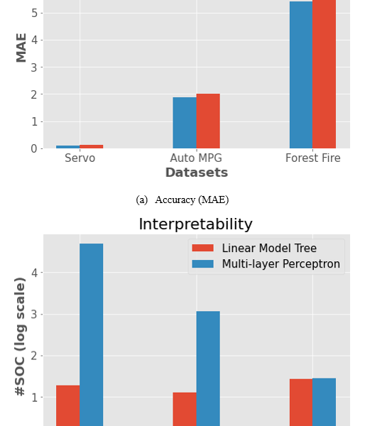
Figure 1: Motivating Example: Accuracy and interpretability of LMT and MLP Algorithms

2.2. Related Work

      Interpretability/explainability of ML models and explainable AI are now emerging research areas due to the wide usage of AI technologies [8]. According to [2], it is favored using simple and interpretable models as they are capable of replacing sophisticated ’black box’ models. In [9], if-then-based rules are extracted from SVM using a two-step method: first run SVM on data and obtain the set of support vectors, then another interpretable model is trained. In [10], the author proposed a human-based proxy metric that is derived from evaluation of model interpretability by humans or a black-box model’s post-hoc interpretation. Authors of [11] studied a simulatability and a ‘what if’ local explainability of logistic regression, neural network and decision tree. They proposed the metric of interpretability as the run time Operation Count (OC). According to [5] the Simulatability Operation Count (SOC) evaluates interpretability for several regression models through the proposed formula. The experiments in this paper use SOC formulas for comparing interpretability of selected models in our experiments.

3. Methodology

3.1.  SOC metric

Interpretability of algorithms can be evaluated in terms of simulatabilty. Simulatability Operation Count (SOC) – the number of arithmetic operations needed to execute an algorithm. According to [8], SOC can be a proxy metric for simulatability. For instance, a linear regression model with 10 variables does 10 multiplications and 9 additions, thus its SOC is 19. More detailed derivation of SOC of estimators can be found in [5].

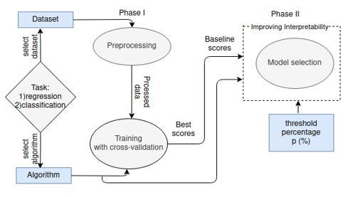
Figure 2: An Overview of the Trade-offs Methodology

3.2.  Workflow of the experiment

The workflow of the experiment is shown in Figure 2. Phase I is divided into Data Preprocessing, followed by Model Training. In the first stage 1) categorical entries of datasets are converted to numerical with OrdinalEncoder [12]; 2) StandardScaler [12] is applied to reduce effects of entries on regression coefficients; 3) outliers which has z-score bigger than 3 are removed from the dataset [13]; 4) correlated entries are dropped to prevent multicollinearity (i.e. Variance Inflation Factor (VIF) is larger than 10) [14]. In the next stage (model training), hyper-parameters are selected by applying GridSearchCV implementation of sklearn [12].

Phase II consists of a model selection method that we are proposing. In the first step, the SOC scores of the chosen estimators at the previous training phase will be evaluated. Next, we repeatedly run a model selection process to decrease SOC scores by letting the accuracy to drop by up to a limit set by threshold percentage (p%) from the highest accuracy values achieved in the training stage (trade-offs between accuracy and interpretability). The threshold percentage is chosen arbitrarily between 0 and 15%, but in reality its optimality depends on the specifics of the task (i.e. error tolerance and requirements like transparency and accountability). For example, on Figure 1a LMT and MLP have almost similar accuracy, on Figure 1b LMT has much lower SOC. In such cases, LMT is a suitable candidate for the tasks that require interpretability of algorithms.

Such trade-off can be done by tuning parameters of models influencing the SOC according to Table 1.

Table 1: SOC formula of algorithms [7]

Estimator		SOC formula
LMT	N/A	2D + 2P + 1
DT	N/A	2D + 1
MLP	Relu Sigmoid Tanh	2 ×  + (2 × + ) ×   = 1 = 4 = 9
SVM	Linear Polynomial Sigmoid RBF	SV × (+ 2) = (2P – 1) = (2P + 1 + d) = (2P + 10) = (3P + 1)

Following the feature selection stage, the number of variables in the dataset (P) is fixed, the depth (D) could be decreased to reduce SOC in Decision Tree (DT) and in LMT.

The type of activation functions (), the number of hidden layers (H) and neurons (N) can be tuned in MLP to obtain lower SOC values. Lastly, selecting a simpler kernel function (, e.g. Linear) and decreasing the number of support vectors (SV) (using NuSVR and NuSVC [12]) and by tuning hyperparameters reduces SOC in SVM.

Table 2: Servo Features

Feature	Description
motor screw pgain vgain class	A,B,C,D,E A,B,C,D,E 3,4,5,6 1,2,3,4,5 0.13 to 7.10

4. Experimental Results

4.1.  Experimental Setup

Datasets for Regression: For our experiments three test datasets (from complex to simple) are used: Forest Fire (complex) [15], Auto MPG (medium) [16] and Servo (simple) [17].

1) Servo: There are 5 variables with target class, and 167 data instances. Value of each variable is discrete, except for the target, it is continuous within the range [0.13, 7.1] and is a servo-mechanism’s raise time. Detailed descriptions are explained in the TABLE 2.

2) Auto MPG: There are 9 variables and 398 data instances, the target variable is ’mpg’ (miles per gallon). Detailed descriptions are in the TABLE 3.

Table 3:  Auto MPG features

Feature	Description
mpg model year cylinders displacement horsepower weight acceleration   origin name	miles per gallon, continuous output variable version of a car power unit of engine measure of the cylinder volume power of engine produces weight of car amount of time taken for car to reach a velocity of 60 miles per hour multi-valued discrete name of the car

3) Forest Fire: There are 517 data instances and 13 vari- ables including a target class ’area’. Full descriptions are in the TABLE 4.

Table 4: Forest Fire features

Feature	Description
area   X,Y month, date   temp, wind, rain RH FFMC,DMC,DC,ISI	in ha, 0 means less than 1ha/100 (=100m2) coordinates of place of fire categorical value from jan. to dec. and mon. to sun. correspondingly meteorological data relative humidity components of Fire Weather Index (FWI) of the Canadian system

Datasets for Classification: The classification datasets include Iris (simple) [18], MNIST (medium) [19] and Pima Indian Diabetes (complex) [20].

4)          Iris: The dataset contains 5 features with 1 target class and 150 instances. Features of Iris dataset are real values and described in TABLE 5.

Table 5: Iris Features

Feature	Description
sepal length sepal width petal length petal width class	1.0 – 6.9 cm 0.1 – 2.5 cm 4.3 – 7.9 cm 2.0 – 4.4 cm Setosa, Versicolour, Virginica

5)             MNIST: The dataset has 784 features and 70000 (60k training and 10k test images) instances, predicting one of 10 digits. Features of MNIST consists of a 28×28 array of real values of all pixels in the picture.

6)             Diabetes: There are 768 instances of 9 features of real values, which are described in TABLE 6. The outcome is positive or negative for the diabetes test.

Table 6: Diabetes Features

Feature	Description
Pregnancies Glucose Blood Pressure Skin Thickness Insulin BMI Diabetes Pedigree Function Age class	0 – 17 0 – 199 0 – 112 0 – 99 0 -846 0.0 – 67.1 0.078 – 2.42 21 – 81 0, 1

Algorithms for Regression: LMT is a model [21] and its implementation was according to M5 design [17]; Scikit- learn library’s [12] MLP Regressor and SVR were used in our experiment. Accuracy metrics is a Mean Absolute Error (MAE)

Algorithms for Classification: DT, MLP Classifier and SVM implementations of scikit-learn library [12] were used to deal with classification task. The percentage of correct predictions (Accuracy) is used as an accuracy metric.

4.2. Results and Analysis

Preprocessing for Regression: Preprocessing stage allowed to reduce Servo dataset to 152 data instances, Auto MPG to 367 (’horsepower’ and ’displacement’ are dropped because of collinearity issue, ’name’ variables is not used), and Forest Fire to 468.

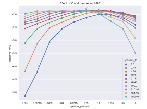
Figure 3: SVR training on Auto MPG dataset.

Model Training for Regression: As mentioned earlier, algorithms are trained with GridSearchCV allowing us to test a broad range of hyper-parameters. Figure 3 shows the process of training SVM on Auto MPG. The lowest error is at C = 1000 and gamma = 0.05 and sub-optimal configuration is obtained by concave down graph.

Table 7: Accuracy Performance (MAE) of Trained Models with references. (Lowest error values in bold).

	Servo                  Auto       MPG       Forest     Fire
LMT MLP SVR Lin. Reg. Other Ref.	0.133                  1.889                      6.847 0.096                  1.890                      5.376 0.183                  1.830                      5.212 0.863                  2.304                      6.723 0.220  [22]         2.020      [23]         6.334      [24]

Overall outcomes of the model training phase are in Table 7. SVR performs better than other models on Auto MPG and Forest Fires datasets and MLP on Servo dataset. Performances of the Scikit Learn’s Linear Regression and other references are provided for comparison.

Model Training for Classification: Like the regression training phase, GridSearchCV is used to find best combina- tions of hyperparameters for the models. One of the examples of parameter-tuning is shown in Figure 4, where optimal values are gamma = 0.00003 and C = 4.64.

Table 8: Accuracy Performance of Trained Models with references. (Highest accuracy values in bold).

	Iris                MNIST              Diabetes
DT Random Forest MLP SVM Other Ref.	96.7%        79.0%                  75.4% 97.7%        97.2%                 76.5% 83.3%        94.9%                  75.7% 98.7%                       96.0%                  77.1% 98.7% [25]   99.7% [26]         76.0% [27]

Training stage’s results are provided in Table 8. On MNIST dataset Random Forest has the best results, while SVM outperforms other models on IRIS and Diabetes dataset. As a comparison, the results of the Random Forest model from the Scikit Learn library were provided.

Model Selection for Regression: Following two approaches to improve interpretability are discussed in this paper: 1) model can be substituted by simpler model and 2) the same model is simplified by tuning its hyperparameters (e.g. reducing the number of neurons or layers in MLP).

Figure 5 shows the results of the first approach and the idea behind it is to demonstrate the behavior of models optimized for interpretability applying the trade-offs method. The point (0, 0) corresponds to the baseline accuracy and SOC score of the estimator on the given dataset. These are the first (top most) entries of each algorithm and dataset pair on Table 9. For example, for LMT and Servo, baseline score is (0.133, 19). The percentage of the increase or decrease is calculated with respect to the baseline score. Next entry in LMT and Servo on Table 9 is (0.134, 17), which corresponds to (0.75 = (0.134 − 0.133)/0.133 × 100, 10.52 = (19 − 17)/19 × 100) point on the blue graph (encircled with red) on Figure 5.

All estimators (MLP, SVR and LMT) behave similarly on regression task. For example, on the Servo dataset SOC is reduced significantly ( approximately by 85%, 17% and 11%) for small raise in error (2.1%, 1.6% and 0.75% respectively). MLP is the most accurate estimator for Servo (with 0.096 MAE value). If 2% reduction in accuracy is feasible for Servo dataset, MLP’s interpretability could be increased by 85%. Alternatively, if MAE value of 0.133 is acceptable for Servo dataset, LMT algorithm with SOC value of only 19 could be used instead of MLP.

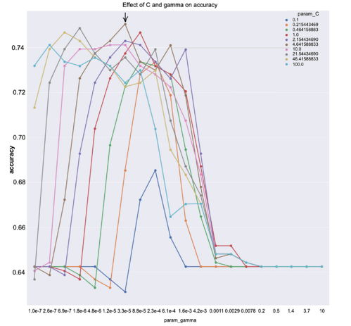
Figure 4: Training SVM on Diabetes dataset.

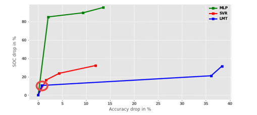
Figure 5: Comparison of Models in Accuracy and Interpretability on the Servo dataset.

Table 9 is a supplement of Figure 5 with additional results of Forest Fire and Auto MPG datasets. Same as in Figure 5, notable advancement is achieved in interpretability with a small degradation in accuracy. For the Auto MPG and Forest Fire datasets using LMT, the most accurate results are obtained with tree depth of 1 (see Figure 7), hence the model cannot be simplified further.

Figure 6 shows the results of the second approach with three datasets using MLP. The similar behavior is observed on all datasets – SOC of the MLP model is decreased notably with small degradation in accuracy. The elbow (turning) points are feasible candidate points for effective trade-off between interpretability and accuracy, since after these points (from left to right) the slopes of the graphs sharply drop. For instance, in Auto MPG dataset (line in red) interpretability is improved (reduction of SOC) by 97% with 2.5% reduction (raise in MAE) in accuracy. The similar pattern is observed in the rest of the datasets.

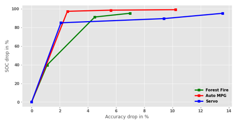
Figure 6: Trade-off between Accuracy and Interpretability in MLP estimator.

Figure 7: Performance of LMT on Forest Fire dataset.

Model Selection for Classification: For the classification task, similar approaches as for regression were applied; and Figure 8 summarizes the results of the first approach where trade-offs between accuracy and interpretability for all the models (DT, MLP and SVM) on MNIST dataset are depicted. It could be seen from Figure 8 that all graphs start at point (0, 0), which are the baseline scores for accuracy and inter- pretability. These baseline score correspond to the last entries (with highest accuracy and SOC values) of each algorithm and dataset pair on Table 10. For instance, for MLP and MNIST baseline score is (94.9%, 10719). Percentage change in SOC or accuracy are calculated with respect to the baseline score, for example, next entry in MLP and MNIST on Table X is (93.4%, 3879), and it gives a red point (1.5% = (94.9% – 93.4%), 64% = (1-(3879/10719))*100 ) on Figure 8. Overall, models perform in the same way on the classification task. For instance, interpretability could be increased dramatically (by 7.3%, 64%, and 40%) in exchange for a small decrease in accuracy (6.62%, 1.5%, and 3.2% correspondingly). SVM is the most accurate model (accuracy 96%) for MNIST dataset, since DT is interpretable intrinsically, its interpretability could not be improved effectively with trade-offs method.

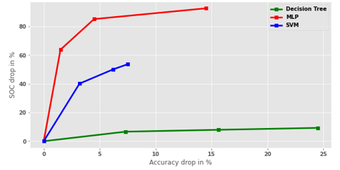
Figure 8: Comparison of Models in Accuracy and Interpretability on the MNIST dataset.

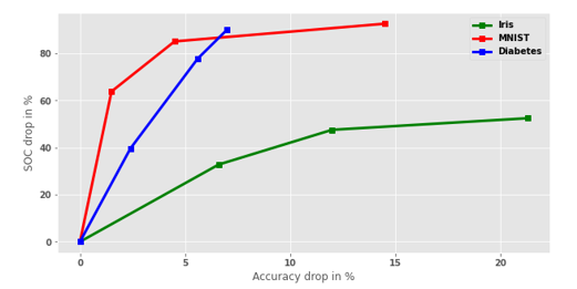
Figure 9: Trade-off between Accuracy and Interpretability in MLP estimator for classification.

Table 10: Comparison of models in terms of accuracy and interpretability (acc. is short for accuracy) for classification.

	DT acc., SOC	MLP acc., SOC	SVM acc., SOC
Iris	66.7%, 11 93.3%, 13 96.0%, 15 96.7%, 17	62.0%, 29 71.3%, 32 76.7%, 41 83.3%, 61	96.7%, 117 97.3%, 162 98.0%, 198 98.7%, 252
Mnist	54.5%, 137 63.4%, 139 71.7%, 141 79.0%, 151	80.4%, 794 90.4%, 1599 93.4%, 3879 94.9%, 10719	88.5%, 45220 89.8%, 48720 92.8%, 58380 96.0%, 97500
Diabetes	72.3%, 19 73.7%, 21 73.8%, 23 75.4%, 27	68.7%, 103 70.1%, 231 73.3%, 627 75.7%, 1038	75.7%, 5185 76.6%, 5338 77.1%,5712 –  –

Table 10 is a more detailed version of Figure 8, and it shows significant increases of interpretability by allowing some drops in accuracy.

The second approach was to test one of the models on three datasets, for example MLP (Figure 9). The model performs similarly on all datasets and SOC could be improved at cost of lowering accuracy. For example, 64% increase of interpretability would require 1.5% reduction in accuracy on MNIST.

5. Conclusion

We introduced a methodology for trade-offs between interpretability and accuracy by inheriting the quantitative and model-agnostic metric – SOC. The LMT model, through its powerful but simple architecture (combination of linear regression and decision tree models), is the most interpretable estimator amongst the considered regression estimators; it has comparable accuracy to MLP in simple-medium datasets like Auto MPG and Servo.

The Decision Tree algorithm has the highest interpretability compared to other evaluated models due to its simplicity on classification task. It outperforms MLP on Iris and shows competitive results on Diabetes dataset. However, it has the lowest accuracy on MNIST with a large gap from other algorithms.

This paper demonstrates the tradeoff method between accuracy and interpretability using SOC metric. SOC is a model agnostic quantitative metric, hence it allows fair comparison between different types of estimators. In our experiments decreasing SOC leads to a simpler model with less memory requirement and faster inference speed. However, in general lower SOC may not always result in models with small memory requirement (i.e. replacing complex operation with simpler one) and faster inference speed (parallelizable model with high SOC can be faster than purely sequential model with low SOC on parallel hardwares).

Conflict of Interest

The authors declare no conflict of interest.

Acknowledgment

This work was partly supported by the Nazarbayev University (NU), Kazakhstan, under FDCRGP grant 021220FD0851.

1. Z. Nazir, D. Kaldykhanov, K.K. Tolep, J.G. Park, “A Machine Learning Model Selection considering Tradeoffs between Accuracy and Interpretability,” 2021 13th International Conference on Information Technology and Electrical Engineering, ICITEE 2021, 63–68, 2021, doi:10.1109/ICITEE53064.2021.9611872.
2. C. Rudin, “Stop explaining black box machine learning models for high stakes decisions and use interpretable models instead,” Nature Machine Intelligence, 1(5), 206–215, 2019, doi:10.1038/s42256-019-0048-x.
3. J.R. Zech, M.A. Badgeley, M. Liu, A.B. Costa, J.J. Titano, E.K. Oermann, “Variable generalization performance of a deep learning model to detect pneumonia in chest radiographs: A cross-sectional study,” PLoS Medicine, 15(11), 1–17, 2018, doi:10.1371/journal.pmed.1002683.
4. C. Molnar, G. Casalicchio, B. Bischl, “Interpretable Machine Learning – A Brief History, State-of-the-Art and Challenges,” Communications in Computer and Information Science, 1323(01), 417–431, 2020, doi:10.1007/978-3-030-65965-3_28.
5. U. Johansson, C. Sönströd, U. Norinder, H. Boström, “Trade-off between accuracy and interpretability for predictive in silico modeling,” Future Medicinal Chemistry, 3(6), 647–663, 2011, doi:10.4155/fmc.11.23.
6. T. Mori, N. Uchihira, “Balancing the trade-off between accuracy and interpretability in software defect prediction,” Empirical Software Engineering, 24, 779–825, 2019, doi:10.1007/s10664-018-9638-1.
7. J.-G. Park, N. Dutt, S.-S. Lim, “An Interpretable Machine Learning Model Enhanced Integrated CPU-GPU DVFS Governor,” ACM Trans. Embed. Comput. Syst., 20(6), 2021, doi:10.1145/3470974.
8. A. Adadi, M. Berrada, “Peeking Inside the Black-Box: A Survey on Explainable Artificial Intelligence (XAI),” IEEE Access, 6, 52138–52160, 2018, doi:10.1109/ACCESS.2018.2870052.
9. M.A.H. Farquad, V. Ravi, S.B. Raju, “Support vector regression based hybrid rule extraction methods for forecasting,” Expert Systems with Applications, 37(8), 5577–5589, 2010, doi:https://doi.org/10.1016/j.eswa.2010.02.055.
10. F. Doshi-Velez, B. Kim, “Towards A Rigorous Science of Interpretable Machine Learning,” ArXiv E-Prints, arXiv:1702.08608, 2017.
11. D. Slack, S.A. Friedler, C. Scheidegger, C.D. Roy, “Assessing the Local Interpretability of Machine Learning Models”, NeurIPS Workshop on Human-Centric Machine Learning, 2019, doi:10.48550/ARXIV.1902.03501.
12. F. Pedregosa, G. Varoquaux, A. Gramfort, V. Michel, B. Thirion, O. Grisel, M. Blondel, P. Prettenhofer, R. Weiss, V. Dubourg, et al., “Scikit-learn: Machine Learning in Python,” Journal of Machine Learning Research, 12, 2012.
13. E-handbook of statistical methods, NIST/SEMATECH, 2012, doi: https://doi.org/10.18434/M32189.
14. R. O’Brien, “A Caution Regarding Rules of Thumb for Variance Inflation Factors,” Quality & Quantity, 41, 673–690, 2007, doi:10.1007/s11135-006-9018-6.
15. P. Cortez, A. Morais, “A Data Mining Approach to Predict Forest Fires using Meteorological Data,” 2007.
16. J.R. Quinlan, “Combining Instance-Based and Model-Based Learning,” in Proceedings of the Tenth International Conference on International Conference on Machine Learning, Morgan Kaufmann Publishers Inc., San Francisco, CA, USA: 236–243, 1993.
17. J.R. Quinlan, “Learning With Continuous Classes,” World Scientific: 343–348, 1992.
18. R.A. FISHER, “THE USE OF MULTIPLE MEASUREMENTS IN TAXONOMIC PROBLEMS,” Annals of Eugenics, 7(2), 179–188, 1936, doi:https://doi.org/10.1111/j.1469-1809.1936.tb02137.x.
19. L. Deng, “The MNIST Database of Handwritten Digit Images for Machine Learning Research [Best of the Web],” Signal Processing Magazine, IEEE, 29, 141–142, 2012, doi:10.1109/MSP.2012.2211477.
20. J. Smith, J. Everhart, W. Dickson, W. Knowler, R. Johannes, “Using the ADAP Learning Algorithm to Forcast the Onset of Diabetes Mellitus,” Proceedings – Annual Symposium on Computer Applications in Medical Care, 10, 1988.
21. L. Dillard, lmt.py, 2017, Link: https://gist.github.com/logandillard/lmt.py.
22. P. Cortez, M.J. Embrechts, “Using sensitivity analysis and visualization techniques to open black box data mining models,” Information Sciences, 225, 1–17, 2013, doi:https://doi.org/10.1016/j.ins.2012.10.039.
23. P.E. Utgoff, ed., “Machine Learning, Proceedings of the Tenth International Conference, University of Massachusetts, Amherst, MA, USA, June 27-29, 1993,” Morgan Kaufmann, 1993, doi:10.1016/c2009-0-27798-1.
24. A. Stanford-Moore, “Wildfire Burn Area Prediction,” 2019.
25. Z. Hussain, H. Ibraheem, M. Aljanabi, A. Ali, M.A. Ismail, S. Kasim, T. Sutikno, “A new model for iris data set classification based on linear support vector machine parameter’s optimization,” International Journal of Electrical and Computer Engineering (IJECE), 10, 1079, 2020, doi:10.11591/ijece.v10i1.pp1079-1084.
26. D.C. Cireşan, U. Meier, L.M. Gambardella, J. Schmidhuber, “Deep, Big, Simple Neural Nets for Handwritten Digit Recognition,” Neural Computation, 22(12), 3207–3220, 2010, doi:10.1162/NECO_a_00052.
27. B. Chandra, V.P. Paul, “A Robust Algorithm for Classification Using Decision Trees,” in 2006 IEEE Conference on Cybernetics and Intelligent Systems, 1–5, 2006, doi:10.1109/ICCIS.2006.252336.

(Click Here)