1. Introduction

Advanced driver assistance systems (ADAS) are multiplying with the emergence of new technologies and the fall in the price of sensors and computers. The ADAS systems not only act on the vehicle in the event of an emergency but also make it easier to drive the vehicle by delegating certain tasks to the vehicle. ADAS are electronic systems that have access to the restitution, traction, braking, and steering components of the vehicle, thus allowing drivers to benefit from assistance and/or to temporarily delegate driving to an automatic co-pilot under certain conditions of traffic [1].

In the literature on driver assistance systems, there are two types: informative systems and active systems. Informative ADAS: Anti-collision system, LDW (Lane Danger Warning), BSD (Blind Spot Detection system), Park assist, and DMS (Driver Monitoring

System). Active ADAS: EBA (Emergency Brake Assist), AEB(Automatic Emergency Braking), VSL (Variable Speed Limiter), VCR (Variable Cruise Regulator), ACC (Adaptive Cruise Control),LKA (Lane Keeping Assist), and LPA (Lane Positioning Assist)[2].

The Lane Danger Warning (LDW) warns the driver in the event of involuntary lane crossing. The device uses for this an infrared sensor or a camera pointed toward the ground in front of the car.

The sensor locates the white lines to the left and right of the vehicle and calculates the relative position of the vehicle in relation to these lines. As soon as the car (bites) the line, an alert is triggered. For this, we were interested in developing this device to create a computer vision radar to take the raw images and then processed, them so that an automatic driving system could be built [3].

Images are important information vectors that represent a considerable amount of data. Their analysis makes it possible to make the decision in terms of space management and locate the areas of interest and carry out processing in real-time [4].

Computer vision tools enable rapid and automatic extraction of qualitative and semantic information, performing relevant information extraction and intelligent interpretation operations on images [5]. For this purpose, the new radars for industrial use or onboard modern cars migrate to the use of computer vision technology thanks to its reliability and cheaper than other types of radars, since they are based on cameras.

In this paper, we present a histogram method processing image data provided by the camera to detect line lanes and compared it with different methods (HOUGH, RANSAC, and RADON) [6], [7]. This paper is organized into 4 sections: In section 1, we present the general processes to detect line lanes. In section 2 we illustrate how to find lanes from the track with the histogram method. In section 3, we present the detection of line lanes by the three methods indicated and their obtained results. In section 4, we compare data from experimental results to the presented methods on videos obtained under real conditions.

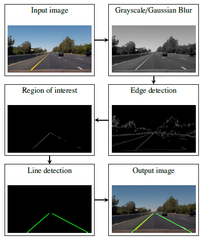
Figure 1: Diagram of the roadway detection & estimation method

2. General approach to the extraction of road marking

In the Figure 1 we illustrate the step-by-step the image processing methodology of the roadway detection and estimation method that achieves the objectives proposed in this paper. This processing is programmed by hybrid languages C++, python-OpenCV, and Matlab.

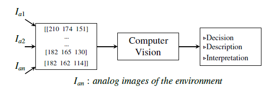
Figure 2: Block diagram of a computer vision system

2.1. Computer vision

The development of computing machines makes it possible to construct a vision system for visual perception capable of naming the objects that surround it, in order to provide the necessary knowledge without ambiguity.

The computer vision system Figure 2 is based on the processing of a sequential sequence of digital images (in the form of pixels) taken by a camera (raw information). Each pixel of the digital image represent an information giving an indication of the amount of light and color coming from the surrounding space [8].

2.2. Frame per second

The general challenge of vision applications is costly in computational time due to the complexity of the algorithms developed. For this reason, the first step to reduce the calculation time is to reduce the processed data depending on time, for this, we have adapted our image capture program to take one image (frame) per second without affecting the data.

2.3. Perspective transformation (Bird-Eye-View)

The Bird-Eye-View transformation technique is to generate a top view perspective of an image, as illustrated in Figure 3. This technique can be classified in digital image processing as a geometric image modification. The Bird-Eye-View transformation can be divided into three stages. First, represented the image in a system of offset coordinates, second rotate the image, third project the image on a two-dimensional plane. The basic diagram of the transformation is given in Figure 4.

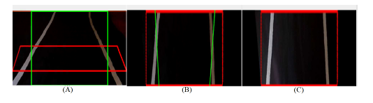
Figure 3: (A) Image originale, (B) Bird-Eye-View image, (C) Output image

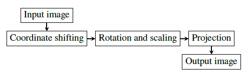
Figure 4: Bird-Eye-View block diagram

2.4. Edge detection

Edge detection is based on Canny Filter, it is a computational approach to detection of marking contours, which represent a fast approach but sensitive to noise because it is accentuated by derivation [9], [10].

After performing a Gaussian smoothing on the image, in order to remove the impurities, then we apply the Canny filter, which calculates the norm of the intensity gradient and the angle of the normal to the gradient (direction of the contours) for each pixel of the smoothed image.

The formulas to apply for each pixel are described as follows:

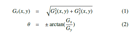
G_y

G_r(x,y) represent the function of the intensities of pixels, in all directions, x and y.

G_x : represents the gradients in x.

G_y : represents the gradients in y.

G_x et G_y are two convolution masks defined previously, one of dimension 3 x 1 and the other 1 x 3:

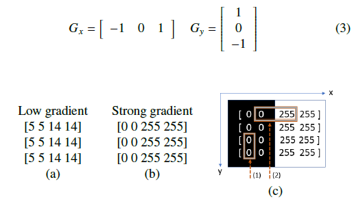
Figure 5: (a) Low gradient. − (b) Strong gradient. − (c) Corresponding image of strong gradient (b). − (1) No change, derivative = 0. − (2) large change, large derivative (gradient).

Canny’s method is based on the derivation variation of G_r(x,y) to determine the image contours, it draws the edge with a big change of intensity (large gradient) and is displayed in the form of white pixel outlines Figures 5 and 6.

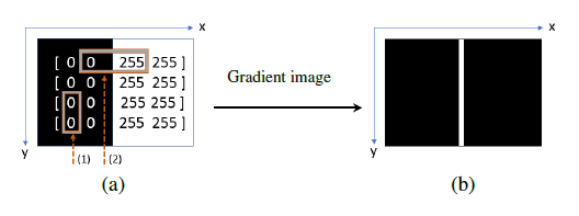
Figure 6: (a) Image. − (1) No change, derivative = 0. − (2) large change, large derivative (gradient). − (b) Image contours in white pixels.

The completely black areas Figure 6(b) correspond to a small variation of intensity between the adjacent pixels. While the white line represents a region of the image where the intensity varies considerably and exceeds the threshold. The threshold is to refine the filtering of the weak contours and to keep only the significant contours, by using two thresholds: High (S _H) and Low (S _L). If the value of a contour is higher than the highest threshold, it is preserved. And if the threshold is lower than the low threshold, the corresponding pixel becomes black.

At this location, two transformations are made of the image obtained after perspective transformation Figure 7(A) to detect the edges, the first is a threshold operation Figure 7(B) and the second is the Canny method Figure7(C). At the end, the two resulting images are confused to guarantee the detection of the edges of the image Figure 7.

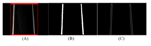
Figure 7: (A) perspective Image, (B) Grayscale image, (C) Canny image

2.5. Region of interest

Automatic detection of the region of interest on an image often has multiple areas is a difficult problem to solve. The proposed method Figure 8 is to determine the region of interest is based on the creation of a digital mask of the image, this mask consists of two types of pixels: 0 represent the black and 255 represent the white, a triangle (or rectangle ) pixels of values 255 identical to the region of interest that we are trying to extract and the rest of the pixels have the value 0 Figure 8(b). The goal is to do the and-logic operation between the bit of each pixel homologous to the image and this mask, thus masking the complex image to show only the region of interest corresponding to the mask Figure 8(c).

And-logical operation

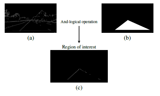
Figure 8: (a) Canny image. − (b) Image mask. − (c) Region of interest.

As the pretreatment steps mentioned and detailed in [8], a region of interest (the red rectangle) is created as illustrated in Figure 9.

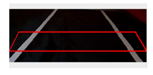
Figure 9: Region of interest

3. Find Lanes from Track using the histogram method

3.1. Histogram method

The histogram method makes it possible to find the exact position of the road line lane from the grayscale image compared to the position of the radar system. This method is based to create a region of interest forms a rectangle in the final image Figures 10(1) and 11(C), divide into different strips.

Algorithm 1: Histogram algorithm

Input : FrameFinal; initialization : DynamicAreas.size(); for int i=0; i < FrameFinal.size().widht ;i++ do RegionOfInterestLane=FrameFinal(rectengle.size()); divide(255, RegionOfInterestLane,

RegionOfInterestLane); push all the intensity valueus in DynamicAreas; histogrameLane.push back(int)(

sum(RegionOfInterestLane)[0] );

end

LeftLaneParametre= max element(histogrameLane.begin(), histogrameLane.lenght()/2);

LeftLanePosition= distance(histogrameLane.begin(),LeftLaneParametre);

RightLaneParametre= max element(histogrameLane.lenght()/2, histogrameLane.end);

RightLanePosition= distance(histogrameLane.begin(),RightLaneParametre);

Output : Final image, LineLanePosition;

In one step, there will be total pixels and each pixel has an intensity of 0 if is black or 255 if is white, we can calculate multiply each step of pixels by its intensity and get the resultant intensity and store this intensity in dynamic areas Figure 10(2), then replace each intensity equal to 255 by X Figure 10(3)(4) and save the coordinates value to find the line lane position. Finally, draw these lines in green and their average on the final image Figure 11(C).

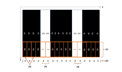
Figure 10: (1) Region of interest, (2) Dynamic areas, (3) Right lane position, (4) Left lane position , (5) Pixels strips

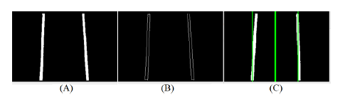
Figure 11: (A) Grayscale image, (B) Canny image, (C) Final image

3.2. Calibrate

We take the average of the lines detected as a reference, it is the instruction of our automatic closed-loop system which must be followed by the car, it is the principle of autonomous driving. Each time the car deviates from this average (the deviation is indicated by a blue line), the system asks to perform the calibration Figures 12, 13 and 14.

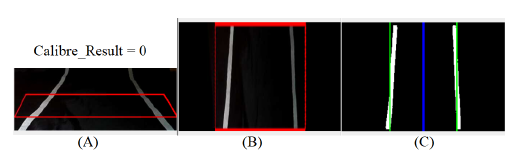
Figure 12: The right position: (A) Original image, (B) Bird eye viw image, (C) Result Image

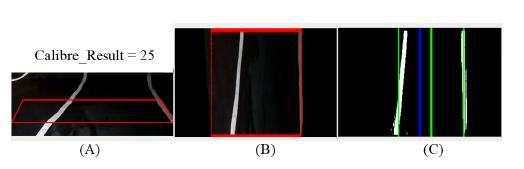
Figure 13: Deviation to the left: (A) Original image, (B) Bird eye viw image, (C) Result Image

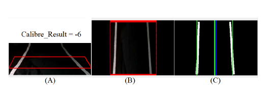
Figure 14: deviation to the right: (A) Original image, (B) Bird eye view image, (C) Result Image

4. Computer vision methods find lanes from the track

4.1. HOUGH Transform

The Hough Transform is an efficient form in recognition tool, the practical application to detect in a camera image the presence of parametric curves from a set of characteristic points, essentially uses the spatial information of the characteristic points, that is, their position in the image. The generalized Hough transform can detect other forms [7].

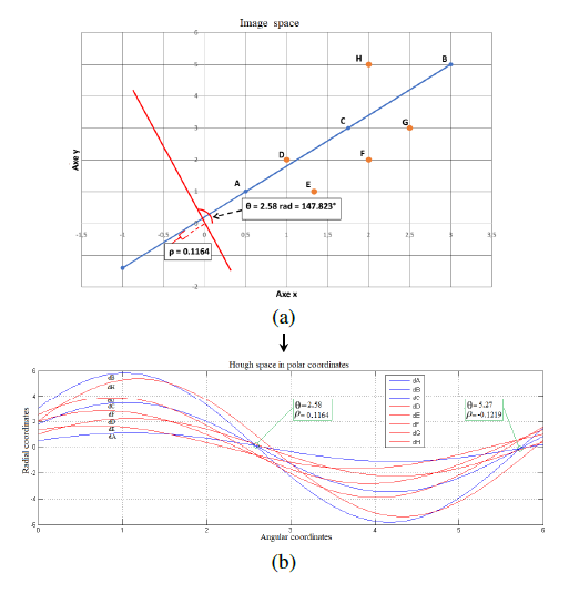
Figure 15: Principle of Polar System. − (a) Distribution of noisy points. − (b) Hough

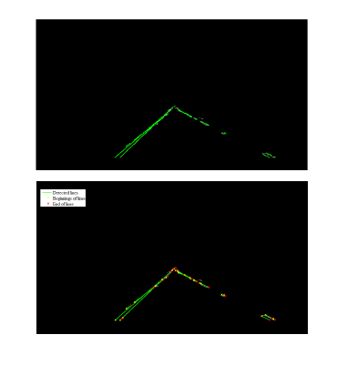
Figure 16: HT Detected lines lanes

The Hough transform algorithm based on the polar system uses an accumulator matrix that represents the space (ρ,θ) [11]–[14], of dimensions (L,C) where L is the number of possible values of ρ and C the number of values of θ. In a distribution of noisy points (x_i,y_j) of the Figure 15(a), each point becomes a sinusoid of the equation “(4)” in the parameter space (ρ,θ). The Figure 15(b) shows, at the end of the accumulation, the sinusoids corresponding to the points of the same line intersect at the point (ρ,θ ) setting this line.

The Figure 16 shows the execution of this algorithm on the image of the regions of interest Figure8(c), so that the accumulator correspond to the votes, which obtained the highest values of the parameters correspond to the lines of the contours of the road way in the treated image.

4.2    Optimization

The detection of roadside contours by the Hough transform is robust as well as the information of the positions of the lines of these contours, this information must be optimized, so that to give a single line in each limit of the road lane Figure 17(a), the objective is to invest in the engineering of Advanced Driver Assistance Systems (ADAS) to build an embedded control system of the vehicle position. The optimization algorithm is summarized in “Algorithm. 2”.

Finally, the experimental results as they appear in the output image Figure 17(b) show that the detection algorithm followed in this paper improves visibility of the roadway and reduces noise.

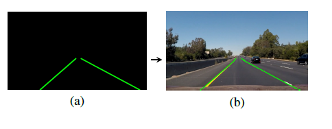
Figure 17: (a) Optimization of line detection. − (b) Output image

Algorithm 2: Optimization algorithm

Slope interception left = [ ]; Slope interception Right = [ ]; for line in linesDET do

% linesDET: the lines detected by the transform;

% each linesDET detected is a 2D array containing the coordinates in [[x1, y1, x2, y2]];

Convert 2D coordinates of linesDET to 1D;

% 2D [[x1, y1, x2, y2]] ⇒ 1D [x1, y1, x2, y2];

Calculate the slope a_i and the interception b_i of each linesDET;

if slope a_i < 0 then

% note that the y axis is reversed. Values increase in descending;

Slope interception left = [a_i,b_i]; else

Slope interception Right = [a_i,b_i]; end

end

Left line parameter = average.(Slope interception left);

Right line parameter = average.(Slope interception Right);

4.3. Probabilistic voting method RANSAC

The robustness of the Radon transform lies in its ability to detect lines in noisy images. Like the Hough transform, it can also

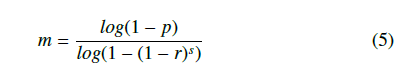
The RANSAC (Random Sample Consensus) method is a probabilism transform lines into easy-to-solve pics that correspond the paramedic voting method based on the use of minimal data to accurately ters of the lines in the outlines of the image. This property of the estimate the parameters of a model, even if the data is noisy. This Radon transform allows us to identify and detect the contour lines method has been proposed to reduce the calculation time of convene of the roadway in the image of the region of interest. After the voting methods such as the Hough Transform. The algorithm optimization, we find very important and valid results Figures 19

of this method is based on a number of iterations, at each turn, it and 20. randomly selects a subset of data (two random points), then finds the model for the selected data, then tests all the data by model and determine the relevant points according to the threshold. In the end, if the new model is better than the best model (based on the number of relevant points), then the new model becomes a best model. From these processes, the estimate preserves the parameters of the searched lines. Let ”p” be the probability of obtaining a good sample, ”s” the minimum number of points in a sample to estimate the parameters of the model and ”r” the probability to have a valid point in all selected contour points. The minimum number ”m” of random draws necessary to have a probability of the correct parameters is as follows:

Finally, in Figure 18 the vehicle circulation lane is determined by exploiting the RANSAC algorithm after 12 iterations, the execution of this algorithm on the same image returns different results because it is based on the random selection of the data, and all the results obtained are valid. The choice of 12 iterations amounts to minimize the calculation time in parallel to obtain a good estimate.

After optimizing the results with the optimization algorithm ”Algorithm. 2”, we obtain a single line in each path limit which is clear in Figure 18(c).

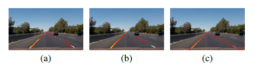
Figure 18: (a) and (b):Track markings detected by our RANSAC algorithm after 12 iterations. (c):Grouping of line segments.

4.4. Radon Transform

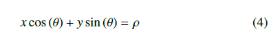
The Radon transform is a mathematical technique developed by Johann Radon, it is defined on a space of lines L in R² according to two arguments (ρ,θ). The application of this transform on a twodimensional function I(x,y) (image) is based on several projections of the image under parallel beams under different given angles, in order to calculate the line integrals of this beam in directions specified. The resulting image R(ρ,θ) of the projection is sum of intensities of the pixels in each direction, can be translated by [15]–[17]:

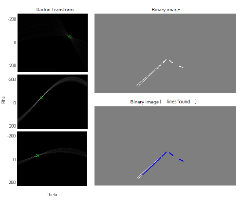
_{Figure 19: Radon algorithm lane detection}

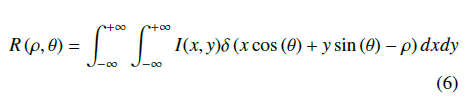
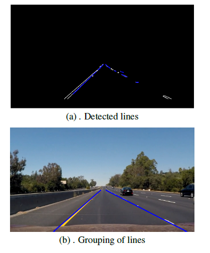
Figure 20: Radon algorithm results

5. Experimental data

We have based on the error (%) (false alarms) of the estimate of the slope and the interception of the detected lines lanes to prove the robustness of the algorithms presented and compare them, by using several tests on sequences of images (videos) of resolution (1280 x 720) in different conditions. Each image sequence has an almost constant width of the line lanes and also has real parameters (slope, interception). The false alarm rate determined after a series of experiments varies acceptably among the four methods compared to the real values Figure 21.

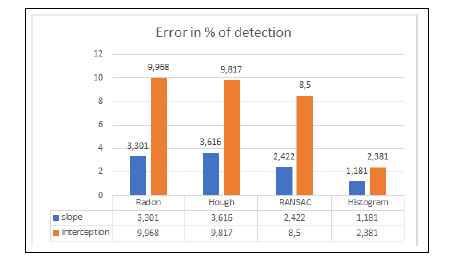
Figure 21: Detection error percentages for each of the four methods

Note, however, that the method based on the histogram presents a minimum error and minimum computing time compared Figure 22 to RANSAC, HOUGH, and RADON methods, due to the data processing being done at the rectangle of the region of interest after generating a perspective view from the above an image.

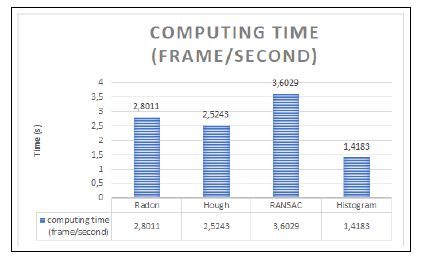
Figure 22: Computing time (frame/second)

6. Conclusion

The comparative study has shown that the proposed vision algorithms (Histogram, Hough, RANSAC, and RADON) are robust to detected contour points with a predefined model describing the curvature of the road, and are quite efficient and have a very efficient accuracy rate despite the fact that noise is present in the images of the road. But the Histogram method presents more efficiency compared to other methods.

The use of these methods is necessary to treat the real environment, but in terms of execution time is very important, which poses a problem of synchronization with the real time of a sequence of images.

In order to complete our study, we want to continue to improve vision algorithms able to be generalized to all roads and detect obstacles and remain robust to different conditions and compatible with real-time processing.

Conflict of Interest

The authors declare no conflict of interest.

1. K. Bengler, K. Dietmayer, B. Farber, M. Maurer, C. Stiller and H. Winner, ”Three Decades of Driver Assistance Systems: Review and Future Perspectives,” in IEEE Intelligent Transportation Systems Magazine, vol. 6, no. 4, pp. 6-22, winter 2014, doi: 10.1109/MITS.2014.2336271.
2. MONOT, Nolwenn. ”From driving assistance systems to connected autonomous vehicles”. 2019. Doctoral thesis in Automation, Production, Signal and Image, Cognitive Engineering. Bordeaux.
3. Rashmi N. Mahajan and Rashmi A. M. Patil, ”Lane departure warning system”. International Journal of Engineering and Technical Research, 2015, vol. 3, no 1, p. 120-123.
4. Charles J.Jacobus, Douglas Haanpaa.:All weather autonomously driven vehicles. U.S. Patent No. 9,989,967. Jun (2018).
5. Monga, Olivier, and Yveline Poncet. ”Computer vision techniques applied to aerial images of floodplains”.(2001).
6. M. A. Rahman, M. F. I. Amin and M. Hamada, ”Edge Detection Technique by Histogram Processing with Canny Edge Detector,” 2020 3rd IEEE International Conference on Knowledge Innovation and Invention (ICKII), 2020, pp. 128-131, doi: 10.1109/ICKII50300.2020.9318922.
7. MAITRE Henri.:A panorama of the Hough transformation. Signal processing. Volume 2 – No.4, pp 305-317 (1985).
8. Hassan Facoiti, Ahmed Boumezzough and Said Safi. ”Comparative study between computer vision methods for the estimation and detection of the roadway”, 2021 7th International Conference on Optimization and Applications (ICOA), 2021, pp. 1-6, doi: 10.1109/ICOA51614.2021.9442633
9. Bassem BESBES, Christele LECOMTE, Peggy SUBIRATS.:New lane line detection algorithm. XXIIe colloque GRETSI, Signal and image processing, September (2009).
10. Canny John.:A computational approach to edge detection. Readings in computer vision. Morgan Kaufmann, pp. 184-203 (1987).
11. Richard O.Duda, Peter E.Hart.:Use of the Hough transformation to detect lines and curves in pictures. No. SRI-TN-36, Communication of the ACM, 15, pp 11-15, janvier (1972).
12. H.Facoiti, S.Safi, A.Boumezzough.:Analyse, caracte´risation et conception d’un syste`me radar anticollision embarque´ dans les ve´hicules. sciencesconf.org:icsat- 2020:326086, pp. 13-18, International Colloquium on Signal, Automatic con- trol and Telecommunications, Caen, France, juin (2020).
13. Simon Haykin.: Neural Networks and Learning Machines. 3rd Edition, New York (2008).
14. Canny John.:A computational approach to edge detection. Readings in computer vision. pp. 184-203 (1987).
15. Jian X.Wu, Sergey V.Kucheryavskiy, Linda G.Jensen, Thomas Rades, Anette Mu¨ llertz, Jukka Rantanen.:Image Analytical Approach for Needle-Shaped Crystal Counting and Length Estimation. Crystal Growth and Design, Bind 15, s.4876-4885 (2015).
16. Hong Wang, Qiang Chen.:Real-time lane detection in various conditions and night cases. Intelligent Transportation Systems Conference, pp. 1226-1231, Canada, September (2006).
17. Kawther Osman, Jawhar Ghommam, Maarouf Saad.:Vision Based Lane Reference Detection and Tracking Control of an Automated Guided Vehicle. 25th Mediterranean Conference on Control and Automation (MED), Valletta, Malta, July (2017).

(Click Here)