1. Introduction

Dealing with the limitations of high-order kinematic redundancy robotic models by advanced control methods has always been focuses of research interests for many years. However, solving the inverse kinematics of these flexible models is not inherently simple, making it even more difficult for models with many degrees of freedom [1], [2]. The same facing issues could be observed in robotic control fields.

To solve the inverse-kinematics problems, many interesting methods have been developed. In [2], a genetic algorithm was employed to minimize both end-effector position errors and joint displacements. Promising control results were obtained, but this algorithm took a long time to search the optimal values. In [3], an intelligent controller was developed for a redundant robot using a null-space approach and Bayesian networks. Mao et al. [4] utilized properties of a multi-layered neural network that could form any continuous nonlinear mapping from one domain to another to design an inverse-kinematics neural network to avoid obstacles and solve different solutions. Implementation time of the biomimetic algorithm [3] was impressively fast while the universal ability was exhibited by the neural approach [4]. The inverse-kinematics problem could be also well treated by various optimization methods such as the stretched simulated annealing (SSA) algorithm [5], and Jacobian pseudo inverse method [6], or the damped least-squares

(DLS) law [7]. However, physical constraints are open issues of these advanced controllers. To cope with these constraint problems, quadratic programming (QP) solutions were derived using optimization algorithms [8]–[9]. By using generic QP solver, it leads to high computation cost and limit the real-time applicability [10]. Another direction for such the constraint problem is the use of null-space constraint remedies [11]. Priority-task vectors could be adopted to specify the task sequence and saturation functions were used as barriers of the constraint violations [12]. Outstanding control performances were produced but the physical constraints were not strictly consolidated in a smooth manner by using these advanced controllers.

To realize high-level control commands, a vast of controllers could be employed such as linear controllers [13], [14] and nonlinear controllers [15], [16]. Between them, sliding mode control (SMC) methods are favorite by researchers and developers thanks to their simplicity, robustness and acceptable working performances [17], [18]. Conventional SMC approaches however only result in infinite control errors [15], [19]. To further improve the control performances, terminal sliding mode control (TSMC) schemes were proposed and effectively applied for a plenty of robotic applications [19], [20]. Nevertheless, singularity problems were observed in the normal TSMC frameworks [21]. Such the weak issues were treated by a nonsingular terminal sliding mode control (NTSMC) methodologies in which the terminal power was taken into account for the time-derivative of the error signals instead of original ones [22]–[23]. However, the use of the NTSMC algorithms leads to dependence of the control signal directly on the time-derivative ones and it could activate vibration phenomena in noisy control cases [24]–[25]. To deal with the NTSMC problem in a comprehensive fashion, new design of the NTSMC is required [22], [26], [27].

This paper is an extension of work originally presented in 2021 International Conference on System Science and Engineering (ICSSE) [1]. In this article, we demonstrate the versatility of the previously mentioned intelligent inverse kinematics solution through its successful application to a 7-DOF redundant robot. Structure of the proposed controller includes two control layers with the following contributions:

1. Robustness of the constrained intelligent inverse-kinematics algorithm in the high-level control layer is improved by the Momentum – Levenberg- Marquardt learning technique.
2. A new nonsingular nonlinear terminal sliding mode control method using a flexible power function is proposed for the low-level control layer to enhance the control performance of the closed-loop system.
3. Effectiveness of the proposed control method is verified by comparative simulation results on a 7-DOF robot model.

The outline of the paper is organized as follows. Section 2 discusses problem statements. The modified design of the intelligent inverse-kinematics algorithm is presented in Section 3. Section 4 shows a new NTSMC controller. The intensive simulation results are presented in Section 5. The paper is then concluded in Section6.

2. Problem Statements

Forward kinematics of a general n-dof robotic manipulator could be obtained using homogenous-transformation computation [5], [6],[7]:

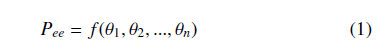
where P_ee ∈ R^N×1 is the end-effector position, θ = [θ₁,θ₂,…,θ_n] is the vector of joint variables, N is the number of task-space variables, and f denotes the forward-kinematics computation.

Behaviors of the joint angles are presented by the following dynamics using the Euler-Lagrange method [28], [27]:

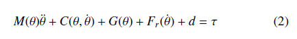
where τ ∈ R^n×1 is the vector of joint torques, M ∈ R^n×n is a symmetric positive-definite mass matrix, C ∈ R^n×1 is the Corioliscentripetal vector, G ∈ R^n×1 is the gravitational vector, F_r ∈ R^n×1 is the Coulomb friction vector, and d stands for external disturbances. Remark 1: Note that with a redundant robot, n is larger than N . We define a position error combining from a desired position P_eed and the system output P_ee. The main control objective here is to figure out proper control signals (τ) to drive the control error to zero complying with specific constraints. To this end, the main controller with a two-layer control structure is used. The complicated dynamics with redundant characteristics and unpredictable external disturbances are however main obstacles in developing the expected controller.

3. High-level Control Layer

The structure of the high-level control layer includes the inverse kinematics solution stage, the constraint integration stage, and the optimization stage.

3.1     A Basic Inverse-Kinematics Method

The main control objective is formulated from the current and desired positions, as follows:

where k•k is the Euclidean norm of the term (•).

By using the Jacobian-transpose-based method to minimize the high-level objective (2), virtual control signal is selected as follows [6], [29]:

where J ∈ R^N×n is the Jacobian matrix of the considering robot, and η is a positive learning constant.

Remark 2: In fact, there are infinite solutions for the problem (3). Hence, it is possible to shape possible solutions inside the expected regions [30].

3.2    Improvements for Joint Constraints

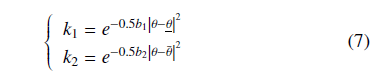
In this subsection, joint constraints are studied as additional control objectives. The former target (3) is modified as:

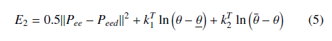
where k₁,k₂ ∈ R^{n ×1} are vectors of positive constants, and (θ,¯ θ) are the upper and lower bounds of joint variables.

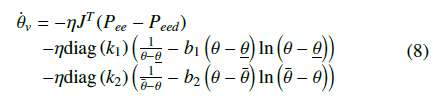
With the new objective (5), the virtual control signal (4) is updated as follows:

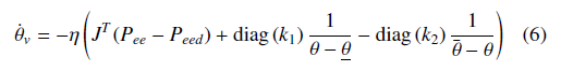
Remark 3: When the function ln is added to the expression (5), it interacts with the angular limit by increasing the value as it gets closer. This means that the virtual speed will also be subtracted a significant amount and has a deceleration effect. The parameter will adjust this interaction amount of the binding component ln.

However, the uncontrolled increase and decrease of this constraint component will adversely affect the real error update and cause large errors for the whole system when working near the hardware limit. The requirement here is that the additional constraint must be large enough to keep the robot within the allowable area and small enough to not affect the error update. Therefore, a new type of the parameter with great flexibility is needed to adjust the constraint up and down properly. Hence, we develop an alternative solution that makes the parameters automatically change under a nonlinear way:

where b_i|i=2,3 are positive constants.

In this virtue, the control signal (6) is updated again as:

Remark 4: At this time, values of the constraint components will be adjusted up by the Gaussian-type gain when the joint variables approach the upper limits or the lower limits. This is caused by the characteristics of the Gaussian function [30], [31] as the variable values approach their centers. Conversely, when the joints move away from the upper and lower limits, depending on the slope of the Gaussian function, the gain will decrease very quickly and push the influence of the constraint down very small. This will satisfy the requirement set forth above.

3.3       Robust Constraint Inverse-Kinematics Approach

From (8), we have reformed the learning of the virtual control signal by using the Momentum-Levenberg–Marquardt method to make it faster while maintaining accuracy:

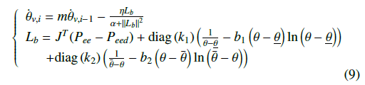
where (0 < m < 1) and α are positive constants, and •_i, •_i−1 denote current and previous states of (•) .

Remark 5: The advantage of this learning algorithm is that it could solve the problems of the normal gradient descent learning methods which are slow to converge and easy to get stuck at the local minimum that is difficult or impossible to reach the global minimum [2], [4], [30]. The Momentum approach could help convergence faster by creating momentum behaviors from the previous velocity, while the shortcoming of instability of Momentum methods would be handled by the Levenberg–Marquardt part due to its ability to damp and ensure all the joint velocities not too different.

4. Finite-time Low-level Control Layer

The low-level control layer is a controller that realize the virtual commands (θ_v) generated by the high-level control one. To control the robot joint (θ) following the desired virtual control signal (θ_v) , we define a low-level tracking control error:

Inspired by terminal sliding mode control theories [17], [18], [19], we then synthesize an indirect control objective as:

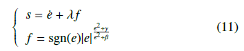
where λ and (γ < β) are positive constants.

To realize the control mission (11) or (12) for the robotic system (10), we propose the following nonlinear terminal control signal:

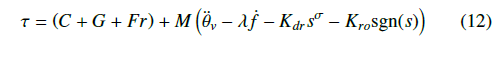
where K_dr, K_ro and (0 < σ < 1) are positive control gains.

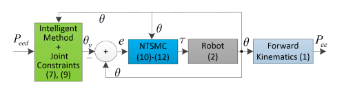
Figure 1: Block diagram of the proposed controller for redundant robots.

Remark 6: The NTSMC method can solve the problem of low settling time and push the error down very small because the larger the error leads to the steeper the selected sliding surface s will be (this is true for both the upper and lower regions of the setpoint); while the steeper the sliding surface provides the faster and more accurate the convergence. This is why the control signal can track the setpoint much better than a Proportional-Integral-Derivative (PID) controller [32], [31]. Block diagram of the proposed controller is presented in Fig. 1.

5. Validation Results

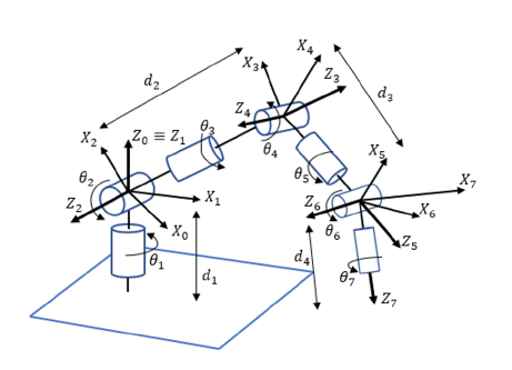
Figure 2: Configuration of a 7DOF robot for investigating.

The proposed controller was verified on a 7DOF redundant robot arm, whose detailed configuration is fully described in Fig. 2. The robot had three links (d₁,d₂,d₃) and seven joints (θ_i|i=1..7). The desired trajectory of the robot was planned in the Cartesian coordinate system O_xyz . The end-effector position P_ee = [x,y,z]^T of the robot is expressed as:

yx==dd−31c(c1c1c6s4(2ss42−()c+d12ss(63s(+4c(5cs(21ccs433(ss1−1)s+c31c−c42scc113sc)22)−c+3cs)16+c(cc415s(s2c2)4s−(4c)d1+s3s3(5c+(6cc(32scs413(+ss11c)s13c−2sc3)))1c2c3)−s1s2s4)+s5(c1c3 − c2s1s3))) +d2(s4(c1s3+c2c3s1)+c4s1s2)+d1s1s2 z=d2(c2c4 − c3s2s4) − d3(s6(c5(c2s4+c3c4s2) − s2s3s5)c6(c2c4 − c3s2s4))+d1c2

where s_i|i=1..₇ := sin(θ_i) and c_i|i=1..₇ := cos(θ_i).

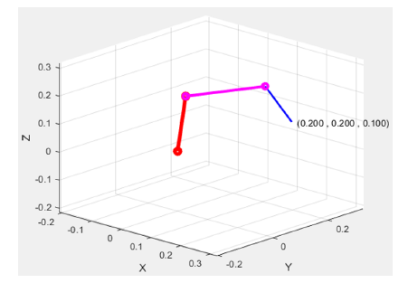
Figure 3: Structure of the 7DOF robot at working position.

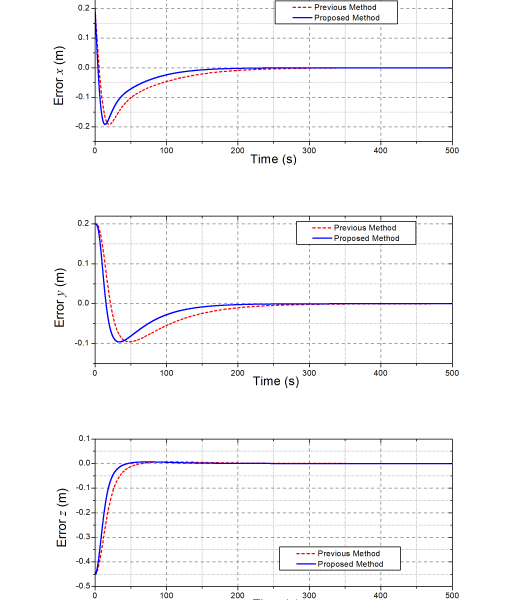
Figure 4: Comparative control errors of the end-effector position obtained by the controllers.

The parameters of the robot model for simulation were selected as follows: m₁ = 0.5 kg, m₂ = 0.5 kg, m₃ = 0.5 kg, m₄ = 0.3 kg, m₅ = 0.3 kg, m₆ = 0.2 kg, m₇ = 0.2 kg, d₁ = d₂ = 0.2 m, and d₃ = 0.15 m . The operating condition was free of interference and had a viscous friction force with a selected friction coefficient µ = 20. The initial values of the joint angles were θ_i|i=1..7 = 0, and the initial end-effector position of the robot in the Cartesian coordinate was (0;0;0.55) (m). The desired position of the end-effector chosen for testing was (0.2;0.2;0.1) (m). To clearly evaluate the control performances of the proposed controller, a previous control method [1] was employed to realize the same control mission in the same system under the same testing conditions. Control gains of the previous controller were selected as b₁ = b₂ = 0.0001,η = diag([0.4,0.4,0.5,0.5,0.6,0.6,0.6]), K_P = 200I₇, K_I = 50I₇, K_D = 25I₇, while those of the proposed controller were manually tuned and obtained as b₁ = b₂ = 0.0001,η = diag([0.4,0.4,0.5,0.5,0.6,0.6,0.6]),α = 1,m =

0.9,λ = 10I7,γi|i=1..7 = 0.95,βi|i=1..7 = 1,σi|i=1..7 = 0.9, Kdr = 100I₇, K_ro = 0.001I₇.

In the first test, the two controllers were applied to control the robot from the initial position to the desired one with the same lowlevel control layer but with different high-level control ones. The response posture of the robot working under the proposed controller after the simulation is shown in Fig. 3. Control results obtained are shown in Figs. 4 – 5.

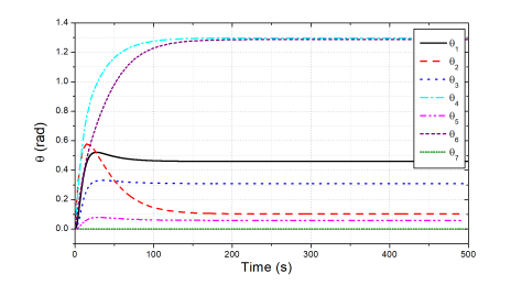
Figure 5: Reference joint angles generated by the proposed controller from the first test.

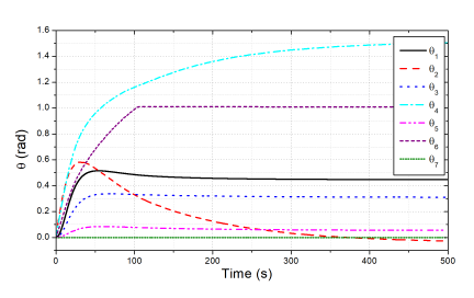
Figure 6: Desired profiles of the joint angles in the joint-constraint test.

The control errors of the end-effector position of the robot accomplished by the two controllers are compared in Fig. 4. Generally, the two control systems were stably working with excellent steady-state control errors of about (6,7.2,4.5) × 10⁻⁶(m) in the x,y,z directions of the end-effector positions, respectively. The figure also shows that the convergence time of the previous controller was about 310 (s) (the red-dot line) while that of the proposed controller was only about 203 (s) (the blue-solid line). The faster results came from the Momentum learning behaviors supported by the Levenberg–Marquardt adaptation scheme (8). Reference joint angles generated by the high-level control layer of the proposed controller are shown in Fig. 5. By combining Figs. 2, 3 and 5, it can be easy to understand that to reach the desired end-effector position, the joints 4 and 6 were hard-working parts with the largest variations ( from 0 to 1.29) (rad).

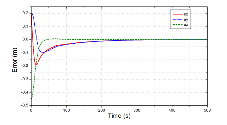
Figure 7: Errors of the end-effector in the joint-constraint test.

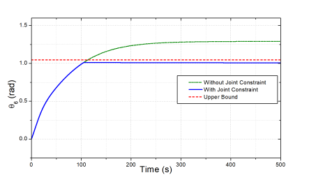
Figure 8: Comparative output at joint 6 in the first and second tests.

To assess the effectiveness of the joint-constraint feature proposed, in the second test, we limited the joint 6 into a range of (−π/3 ≤ θ₆ ≤ π/3) . The simulation results achieved by the proposed controller for the old and new testing conditions are presented in Figs. 6-8. As seen in Fig. 7, the proposed controller still ensured the excellent control quality for the end-effector positions under the constrained working condition. Furthermore, as shown in Fig. 6, the profiles of all joint angles would also change to ensure that the data changes of θ₆ was still inside of the given range (−π/3;π/3). The profiles of the joint variable θ₆ in this test and the last test are compared in Fig. 8. It can be seen that, in the case of the constraint defined, the angle θ₆ increased very fast to the upper limit and then stopped increasing and kept a certain distance with the upper limit because the joint velocity was greatly reduced caused by the algorithm. The results would also be similar for the other joints if other joint constraints were applied. Note that, thanks to the redundant robot configuration possessed, even though the joint angle θ₆ was limited, the control burden was shared by the other joint angles, especially by the joint θ₂ and θ₄, that could be observed in this test by comparing the data in Figs. 5 and 6.

In the third test, we performed a new simulation to show the importance of the low-level control layer by comparing the response quality between the new controllers with NTSMC and previous PID controllers [1]. The two controllers were used to control the end-effector of the robot to the desired position and their control results are compared in Figs. 9-12. For the easier observation, we only took the results of joints 2, 4, 6 because they are folded joints.

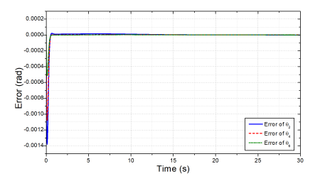
Figure 9: The joint control errors obtained by the new NTSMC controller.

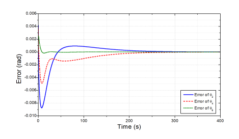
Figure 10: The joint control errors obtained by the previous controller.

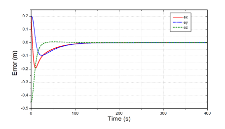
Figure 11: The end-effector control errors obtained the proposed controller.

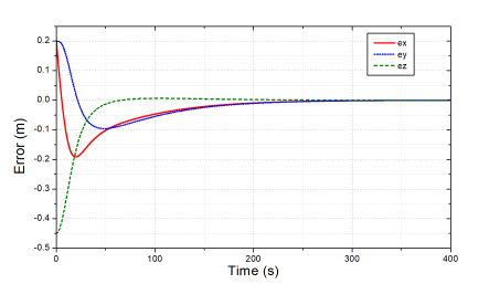
Figure 12: The end-effector control errors obtained the previous controller.

The results in Figs. 9 and 10 indicate that the settling time and the transient response of the new controller were superior to those of the old one (ten times faster). Achieving a very small error (±10⁻⁴) in a very short time has shown the effectiveness of the improved NTSMC method compared to the previous one. The other control results in Figs. 11 and 12 also imply that with the improvements in the low-level control layer, it is not surprising about the faster response and higher accuracy in the end-effector control space obtained by the proposed controller as comparing to the previous one.

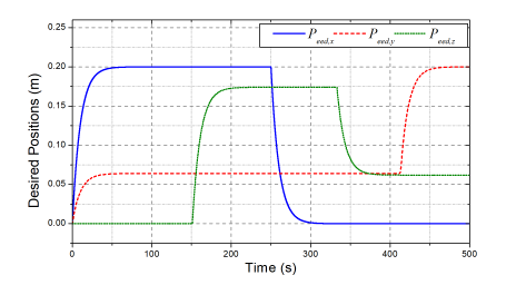
Figure 13: The desired end-effector positions in the fourth test.

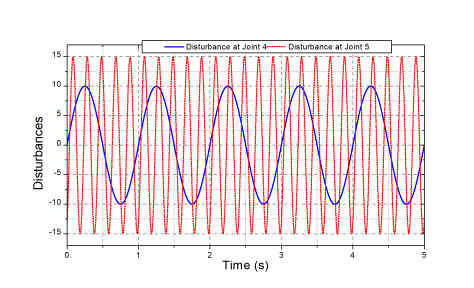
Figure 14: External disturbances in the fourth test.

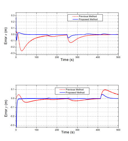
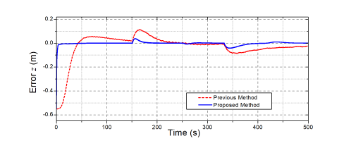
Figure 15: Comparative control errors at the end-effector of the robot.

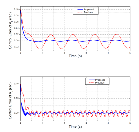
Figure 16: Comparative control errors of the robot joints.

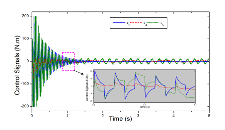
Figure 17: Control signals generated by the proposed controller at the robot joints.

To validate the feasibility of the proposed control approach, in the last simulation, the robot was challenged with new desired endeffector positions of multi-step signals, as depicted in Fig. 13, and external disturbances at joints 4 and 5 as presented in Fig. 14. The obtained control results of the proposed and previous controllers are illustrated in Figs. 15 – 17. Under the new testing conditions, as seen in Fig. 15, the designed controller still provided higher control accuracies and faster settling time at the end-effector than the previous one. To this end, the proposed control approach was not only employed the robust intelligent learning control law (7)-(9) but it was also supported by the new NTSMC framework (10)-(12).

Indeed, as shown in Fig. 16, the control errors of the new nonlinear low-level controller at joints 4 and 5 in the heavy disturbances were respectively 0.0018 (rad) and 0.002 (rad), while those of the previous one were 0.03 (rad) and 0.015 (rad). Figure 17 shows the control signals generated by the proposed controller. The feasibility of the proposed control method could be confirmed throughout the data obtained.

6. Conclusions

In this paper, an intelligent two-layer control method for dealing with inverse-kinematics problems of redundant robots has been improved and applied to a 7-DOF robot. In the high-level control layer, the inverse kinematics problem is solved by using the Momentum-Levenberg optimization method. In cases of the joint constraint requirements, an advanced constrained learning feature can be activated to ensure that the robot joints can avoid physical limit collisions. To enhance the control performance of the overall system, a new nonlinear terminal sliding mode control framework is developed in the low-level control layer. The effectiveness of the proposed control algorithm has been consolidated by comparative validation results obtained. In the future, the intelligent method will be integrated more advanced, optimal, flexible working features and verified on a real-time system.

Conflict of Interest

The authors declare no conflict of interest.

1. D. M. Hung, D. T. Linh, D. X. Ba, “An Intelligent Control Method for Re- dundant Robotic Manipulators with Output Constraints,” in 2021 International Conference on System Science and Engineering (ICSSE), 116–121, 2021, doi:10.1109/ICSSE52999.2021.9538490.
2. A. C. Nearchou, “Solving the inverse kinematics problem of redundant robots operating in complex environments via a modified genetic algo- rithm,” Mechanism and Machine Theory, 33(3), 273–292, 1998, doi:10.1016/ S0094-114X(97)00034-7.
3. P. K. Artemiadis, P. T. Katsiaris, K. J. Kyriakopoulos, “A biomimetic approach to inverse kinematics for a redundant robot arm,” Autonomous Robot, 29, 293–308, 2010, doi:10.1007/s10514-010-9196-x.
4. Z. Mao, T. C. Hsia, “Obstacle avoidance inverse kinematics solution of re- dundant robots by neural networks,” Robotica, 15, 3–10, 1997, doi:10.1109/ ROBOT.1993.291813.
5. P. Costa, J. Lima, A. I. Pereira, P. Costa, A. Pinto, “An Optimization Approach for the Inverse Kinematics of a Highly Redundant Robot,” in Abraham, A., Wegrzyn-Wolska, K., Hassanien, A., Snasel, V., Alimi, A. (eds) Proceedings of the Second International Afro-European Conference for Industrial Advance- ment AECIA 2015. Advances in Intelligent Systems and Computing, volume 427, 433–442, 2015, doi:10.1007/978-3-319-29504-6 41.
6. D. X. Ba, J. B. Bae, “A precise neural-disturbance learning control of con- strained robotic manipulators,” IEEE Access, 9, 50381–50390, 2021, doi: 10.1109/ACCESS.2021.3069229.
7. D. S. Binh, K. L. Thanh, D. P. Nhien, D. X. Ba, “An intelligent inverse kinematic solution of universal 6-DOF robots,” in Huang, Y. P., Wang, W. J., Quoc, H.A., Giang, L.H., Hung, N.L. (eds) Computational Intelligence Methods for Green Technology and Sustainable Development. GTSD 2020. Advances in Intelligent Systems and Computing, volume 1284, 107–116, 2020, doi:10.1007/978-3-030-62324-1 10.
8. F. Cheng, T. Chen, Y. Sun, “Resolving manipulator redundancy under inequal- ity constraints,” IEEE Transactions on Robotics and Automation, 10(1), 65–71, 1994, doi:10.1109/70.285587.
9. A. Escande, N. Mansard, P. B. Wieber, “Fast resolution of hierarchized inverse kinematics with inequality constraints,” in 2010 IEEE International Conference on Robotics and Automation, 3733–3738, 2010, doi:10.1109/ROBOT.2010. 5509953.
10. A. Escande, N. Mansard, P. B. Wieber, “Hierarchical quadratic programming: Fast online humanoid-robot motion generation,” The International Journal of Robotics Research, 7(33), 1006–1028, 2014, doi:10.1177/0278364914521306.
11. F. Flacco, A. D. Luca, O. Khatib, “Prioritized multi-task motion control of redundant robots under hard joint constraints,” in 2012 IEEE/RSJ Interna- tional Conference on Intelligent Robots and Systems, 3970–3977, 2012, doi: 10.1109/IROS.2012.6385619.
12. F. Flacco, A. D. Luca, O. Khatib, “Control of redundant robots under hard joint constraints: saturation in the null space,” IEEE Transactions on Robotics, 31(33), 637–654, 2015, doi:10.1109/TRO.2015.2418582.
13. V. I. Utkin, “Sliding mode control design principles and applications to elec- tric drives,” IEEE Transactions on Industrial Electronics, 40(1), 23–36, 1993, doi:10.1109/41.184818.
14. J. Zhang, W. X. Zheng, “Design of adaptive sliding mode controllers for linear systems via output feedback,” IEEE Transactions on Industrial Electronics, 61(7), 3553–3562, 2014, doi:10.1109/TIE.2013.2281161.
15. D. X. Ba, “A Fast Adaptive Time-delay-estimation Sliding Mode Control for Robot Manipulators,” Advances in Science, Technology and Engineering Systems Journal, 5(6), 904–911, 2020, doi:10.25046/aj0506107.
16. C. Hu, B. Yao, Q. Wang, “Performance-oriented adaptive robust control of a class of nonlinear systems proceeded by unknown dead zone with compara- tive experimental results,” IEEE/ASME Transactions on Mechatronics, 18(1), 178–189, 2013, doi:10.1109/TMECH.2011.2162633.
17. Z. H. Man, A. P. Paplinski, H. R. Wu, “A robust MIMO terminal sliding mode control scheme for rigid robot manipulator,” IEEE Transactions on Automatic Control, 39(12), 2464–2469, 1994, doi:10.1109/9.362847.
18. L. Fridman, J. Moreno, R. Iriarte, Sliding Modes after the first Decade of the 21st Century, Springer Berlin, Heidelberg, 2012, doi:10.1007/ 978-3-642-22164-4.
19. S. T. Venkataraman, S. Gulati, “Control of nonlinear systems using termi- nal sliding modes,” in 1992 American Control Conference, 891–893, 1992, doi:10.23919/ACC.1992.4792209.
20. Y. Tang, “Terminal sliding mode control for rigid robots,” Automatica, 34(1), 51–56, 1998, doi:10.1109/9.362847.
21. K. B. Park, J. J. Lee, “Comments on ‘A robust MIMO terminal sliding mode control scheme for rigid robotic manipulators,” IEEE Transactions on Auto- matic Control, 41(5), 761–762, 1996, doi:10.1109/9.362847.
22. D. X. Ba, H. Yeom, J. B. Bae, “A Direct Robust Nonsingular Terminal Sliding Mode Controller based on an Adaptive Time-delay Estimator for Servomotor Rigid Robots,” Mechatronics, 59, 82–94, 2019, doi:10.1016/j.mechatronics. 2019.03.007.
23. C. K. Lin, “Nonsingular terminal sliding mode control of robot manipulators using fuzzy wavelet networks,” IEEE Transactions on Fuzzy Systems, 14(6), 849–859, 2006, doi:10.1109/TFUZZ.2006.879982.
24. Z. Ma, G. Sun, “Dual terminal sliding mode control design for rigid robotic manipulator,” Journal of the Franklin Institute, 355(18), 9127–9149, 2018, doi:10.1016/j.jfranklin.2017.01.034.
25. R. M. Asl, Y. S. Hagh, R. Palm, “Robust control by adaptive nonsingular terminal sliding mode,” Engineering Applications of Artificial Intelligence, 59, 205–217, 2017, doi:10.1016/j.engappai.2017.01.005.
26. Y. Shtessel, M. Taleb, F. Plestan, “A novel adaptive-gain supertwisting sliding mode controller: Methodology and application,” Automatica, 48(5), 759–769, 2012, doi:10.1016/j.automatica.2012.02.024.
27. J. Baek, M. Jin, S. Han, “A new adaptive sliding mode control scheme for application to robot manipulators,” IEEE Transactions on Industrial Electronics, 63(6), 3628–3637, 2016, doi:10.1080/00207179308934387.
28. Y. Feng, X. Yu, Z. Man, “Nonsingular terminal sliding mode control of rigid manipulators,” Automatica, 38(12), 2159–2167, 2002, doi:10.1016/ S0005-1098(02)00147-4.
29. O. Kanoun, F. Lamiraux, P. B. Wieber, “Kinematic control of redundant manipulators: Generalizing the task-priority framework to inequality task,” IEEE Transactions on Robotics, 27(4), 785–792, 2011, doi:10.1109/TRO.2011.2142450.
30. A. Tringali, S. Cocuzza, “Globally Optimal Inverse Kinematics Method for a Redundant Robot Manipulator with Linear and Nonlinear Constraints,” Robotics, 9(3), 2020, doi:10.3390/robotics9030061.
31. E. Krastev, “Sliding Mode Control of a Redundant Robot Arm in Motion Planning Subject to Joint Space Constraints,” in 2017 International Conference on Control, Artificial Intelligence, Robotics and Optimization (ICCAIRO), 109–114, 2017, doi:10.1109/ICCAIRO.2017.31.
32. C. M, W. Xu, C. Sun, “On switching manifold design for terminal sliding mode control,” Journal of the Franklin Institute, 353, 1553–1572, 2016, doi: 10.1016/j.jfranklin.2016.02.014.

(Click Here)