1. Introduction

Detecting and Identifying building locations is vital for varieties of applications such as mapping, military situations (active engagement of forces, counter-terrorism and peacekeeping measures), natural disaster management (flooding, earthquakes, and landslides), environmental preparation, and urban planning [1–6]. It is feasible to distinguish buildings from the images; however, this can be a time-consuming or difficult operation. Therefore, Automatic building extraction from aerial or satellite images is a highly needed and challenging problem due to its complexity. Moreover, with the advanced technology of capturing very high spatial resolution imagery and the increasing need for map revision without the high cost and time-consuming as a consequence of the rapidly growing urbanization. Automatic building detection becomes possible as the ground resolution size of the pixels is much smaller than the average size of objects in those images. During the past decade, many studies have been carried out on building extraction [7–9]. However, it is still difficult to detect buildings in urban areas because of their variety of shapes, sizes, colors, textures, and the similarity between building and non-building objects.

In the field of building detection, most methods have been based on artificial features; like in work [10], due to low-quality RGB geophotos and to reduce the problem of characteristics extracted from those images, they used the Haar feature method to be able to apply machine learning techniques on it. As for work [11], it integrates a set of algorithms inspired by the human visual system with a combination of classical and modern approaches for extracting image descriptors. Then, the feature descriptors are processed with machine learning to identify buildings.

 Moreover, Deep learning-based approaches have been proposed recently. Including, In [12] focused on three different ways to use convolutional neural networks for remote sensing imagery. The authors suggested [13]a set of convolutional neural networks for township building identification that can be applied to a pixel-level classification framework. In [14] proposed a general framework for convolutional neural network-based classification. In [15], a building extraction framework is proposed based on a convolutional neural network (CNN), edge detection algorithm, and building structure. The masked R-CNN Fusion Sobe framework was used to extract the building from high-resolution remote sensing images. But the results showed that it works poorly to extract edges and preserve the building instances’ integrity.

However, These studies are not without their limitations, especially since CNN cannot successfully learn the features of the hierarchical contextual image due to the lack of data sets, and increasing the number of layers in the deep model leads to more significant training mistakes. CNNs’ prediction abilities with less computation come at the cost of reduced output accuracy.

This paper focuses on building detection from 2D aerial (or satellite) imagery. Therefore a novel approach addresses two main issues: (a) the problem with the particular colors for some buildings with a similar color to other objects in urban images, and (b) the difference in color shades on building’s rooftops. The paper is organized in the following way: The related work section categorizes and presents works that tackle the issue of building detection. Section 3, details the steps that have been applied to classify the image into four classes. Then in section 4, we describe how to accurate buildings positions. And section 5, shows the results provided by our experiments and a comparison with some other works. Finally, conclusions and perspectives for future work are in section 6.

2. Related Work

As we said before, building detection is one of the most difficult challenges to solve since they have so many different properties. Numerous building detection techniques have been presented throughout the years, having their efficacy measured in various ways. In this section, we review works that attempt to solve those challenges. Most of those researches can be classified according to whether they are supervised or automatic, extract geometric features, or are area-based [16]. Another classification is based on the use of the height data, the simple 2D imagery, or a hybrid [17].

In [8], the authors proposed an automatic approach using level set segmentation constrained by priors known shape models of buildings. In [18], the authors presented a supervised model using the active contour method combined with local texture and edge information by initial seed points on one of the buildings. The authors [16] have developed an automatic tertiary classifier to identify vegetation, buildings, and non-buildings objects using Nadir Aerial Image with one condition that the building has a convex rooftop. They reduce the colors from 255 for each RGB channel to 17. Then, using segmentation and thresholding on the green color channel to identify the vegetation regions and on the difference between the blue and green color channels to identify shadows. Finally, buildings and non-building are detected by measuring the solidity of their regions using the entropy filtering and watershed segmentation. In [19], the authors present an automatic technique using LIDAR data and multispectral imagery. Buildings and trees are separated from other low objects using thresholding for height. After that, they eliminate the trees with the normalized difference vegetation index method from an orthorectified multispectral image. The authors proposed [20] an automatic approach using a digital surface model and multispectral orthophoto. Initially, they created a building mask from the normalized digital surface model that included only areas where the possible locations for buildings. Then, the vegetation was separated from the building mask using a modified vegetation index based on the use of the near-infrared orthophoto and the correction of the vegetation index using the shadow index and the texture analysis. Finally, using Radon transform, they extract the building position. In [21], the authors implement an object-based classification for urban areas using spot height vector data. After the segmentation of the image, they had classifier the obtained result into five class vegetation, shadows, parking lots, roads, and buildings based on the analysis of the combined spectral, textural, morphological, contextual, and class-related features to assign a class membership degree to each segment (object) based on membership functions or the thresholds. In [22], the authors implemented an automatic method based on the similarity between building roofs using a previously defined reference set to generate a grayscale image with an enhanced potential for building location. Then, they assign pixels to possible buildings or nonbuilding locations using the hit-or-miss transform morphology. Finally, after defining the shadow areas, they verified the final location of the buildings. In [23], the authors developed a supervised approach based on shadow position using segmentation and classification of color features. First, they split the image into superpixel patches with the segmentation algorithm. After that, using Linear discriminate analysis (LDA) color features and support vector machines (SVM) with a previous set of chosen patches for three classes: buildings, non-buildings, and shadow. Finally, from the prior knowledge of the shadows’ position, they define a seed point location, and with the regional growth method, they determine the positions of the buildings. In [24], the authors proposed an automatic approach based on the rectangle form of the buildings. They enhance the edge contrast using a developed bilateral filter. Then, they apply a line segment detector to extract lines. Finally, a perceptual grouping approach groups previously detected lines into candidate rectangular buildings. In 2016 [25], the authors provided an ontology-based system for slum identification based on the built environment’s morphology. In this technique, a segmentation is followed by hierarchical classification utilizing object-oriented image analysis. For each object, spectral values, form, texture, size, and contextual connections are all computed based on the purpose of the classification. In [26] adopt a new object-based filter consisting at first of splitting the image into homogeneous objects using multi-scale segmentation and at the same time extracting their features vector. Considering that each splitter object is in the center of his surrounding adjacent objects and a part of a fully real existing object in the image. Then, there are two possibilities of his location, either in the interior or in the real object. Hence, it has similar features to its surrounding adjacent objects or in the boundary with no similarity between them.  Therefore, topology and feature constraints are proposed to select the considered adjacent objects. Finally, the feature of the central object is smoothed by calculating the average of the selected object’s feature. In [27], detecting buildings by determining them using a one-class SVM, They proceed with the texture segmentation technique using a conditional threshold value to extract buildings of different colors and shapes. Buildings are identified from the rest of the roads and vegetation regarding the angle of shadows. In [28], the Building Detection with Shadow Verification (BDSV) approach was introduced, integrating multiple features such as color, shape, and shadow to detect buildings. Because some roofs can be extracted with color features only, such as for buildings with sloped roof tiles, while Non-tile flat roofs depend on the shape features. The shadow properties were also incorporated, (Candidate buildings with close shadows will be considered as actual buildings).

Nonetheless, many challenges remain to be overcome in building extraction. To begin with, some of the buildings have a particular color (green, red…), so the approaches based on color classification can’t separate buildings from trees or lawns [16,17,19,20,23]. Rather than assume that buildings have a standard form like rectangles or use a predefined shape database to bring the results closer to a particular format [8,24], we can’t cover all those possibilities of their forms. Furthermore, others use texture to solve the color problem. Yet, they only use it to calculate the entropy or the homogeneity of a single-pixel combined with the high data of objects or to detect the whole area of buildings without separating one from another [21,25]. Therefore, those methods can’t give us the results we request without the high data or in a complex scene. That being the case, can we benefit from segmentation to a superpixel size unity by applying the texture methods on the entire superpixel, assuming that they are small-sized objects rather than on a single pixel?.

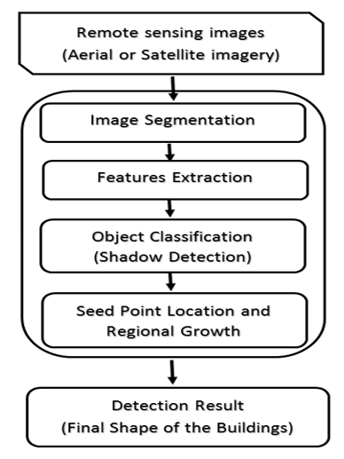
Figure 1. Diagram flow of the proposed algorithm.

3. Classification of image data

Most urban images have six kinds of land covers: trees, grass, shadows, roads, parking lots, and buildings. Trees and grass are usually green, but this depends on the type and the season the image was taken (they may be in red or yellow). Roads and parking lots have, in general, a gray color; unlike the shadows, areas are darker or completely black. And finally, buildings have different color rooftops based on the image’s location (the diversity of culture, climatic nature…). In Figure 2, various structures, building patterns, lighting conditions, landscape characteristics, and complex buildings are located within the study area. Visual inspection can quickly discover complicated patterns in buildings, but machine learning cannot.

Consequently, buildings may have a color similar to trees or roads and parking lots. Therefore, we relied on two things to solve this problem: (a) the shadow factor to separate buildings from roads and parking lots, and (b) for trees, the texture features can do the trick. As a result, according to color and texture, four classes pop up: the first one contains buildings, the second is trees and grass, the third are roads and parking lots, and finally shadows. So, to obtain those classes, three steps have been taken into account, We’ll walk through them in detail:

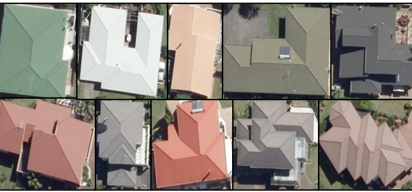
Figure 2: Aerial images of buildings in the study area New Zealand from various perspectives

3.1.  Superpixel Segmentation Using SLIC

Superpixel segmentation divides an image into a group of connected pixels with similar colors. Instead of working with pixels in a big-sized image, we can reduce it into superpixel patches without losing too much information. The Simple Linear Iterative Clustering (SLIC) algorithm for superpixel segmentation proposed in [29] is a k-means-based local clustering of pixels in the 5-D space [l, a, b, x, y], where (l; a; b) is the CIELAB color space and (x; y) is pixel coordinates. SLIC adapts the k-means clustering approach to efficiently generate superpixels introducing a new distance measure D_s as described in Eq. [1].

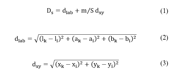
where k and i are respectively the indices of the superpixels center and their surrounding pixels, m is a variable that allows controlling the compactness of superpixels, and S is the grid interval between them.

In consideration of the foregoing, this step aims to have homogenous superpixels as much as possible with a sufficient size that allows us to extract texture features disregarding the shape of each one of the superpixels. Therefore, a high value of m makes the spatial distances outweigh the color factors giving more compacted set-sized superpixels that lead to disrespecting the boundaries of the objects in the image. The other way around for a lower value, this will produce small sizes superpixels. So, To get effective results, we chose a low-value number. Then, merge each superpixel with a smaller size than a given thresholding number of pixels to the nearest similar neighbor. It will turn them into one larger superpixel without losing the adherence to object boundaries.

3.2.  Texture Features Extraction Using (ICICM)

Color co-occurrence matrix (CCM) is one of the most efficient yet straightforward texture descriptors. It consists of extracting statistical measurements about the co-existence of different colors from the image. Integrative Color Intensity Co-occurrence Matrix (ICICM) has been introduced in [30] as an extension of CCM to simulate the human perception of textures. They argued that each pixel might be regarded as color or gray-level depending on its intensity level. Thus, two measures, namely W_col and W_gray, which determine the extents of color and gray, have been extracted from each pixel within the image. After that, these measures have been used to extract four co-occurrence matrices that represent the co-existence of W_col / W_col, W_col = W_gray, W_gray=W_col, and W_gray = W_gray. Finally, a set of third-order statistical moments have been drawn and used as image descriptors. An improvement of ICICM has been proposed in [31], in which a smooth approach of color/gray-level space quantization has been adopted. Ultimately, ICICM has been used to extract texture features for each final form superpixel.

3.3.  Identifying Classes Using SVM

A Support Vector Machine (SVM) is a supervised discriminative classifier formally defined by a separating hyperplane. Given a set of training examples with which class they belong, the SVM training algorithms create a model that can assign the new data to one of those classes. Therefore, the SVM classifier can be trained with the combination vectors between the LAB color features and the texture features of the training superpixel samples to obtain our final class results. The samples are taken from each of the four classes, a simple linear kernel type of SVM was applied, and the results are shown in figure 3(d).

4. Accurate Building Position

From the previous results in figure 3(d), we can see that buildings and trees are entirely separated, unlike some similarities with the roads and the parking lots. As we mentioned before, the prior knowledge of the direction of the shadows lets us distinguish between elevated objects and the ones at ground level. Still, the problem is how to detect the exact shape of the buildings.

Usually, the rooftop of the building has the same color; therefore, a seed point location with the regional growth method may do the trick. However, in many areas around the world and depending on the designs of the buildings, it can cause to show darker sides than the others on the rooftop of the buildings, so we adept our new implementation of the regional growth to resolve this problem.

4.1.  Seed Point Location and Regional Growth

At first, an initial superpixels seed points location is defined based on three conditions:

• the superpixels in the shadows class and have a neighbor from the trees class are eliminated;
• the superpixels that have been considered as seed points must be in buildings class that is a neighbor to the one in shadows class after the elimination according to their respective direction (in this case, the up and right sides);
• The superpixels with more neighbors from road class than building class are eliminated.

Next, to make sure that the seed points are located all over the region of the building and resolve the darker side problem, we applied the regional growth method using the [a, b, ep, h, c, en] vector with the earlier initial superpixels seed points where a and b are the green–red and blue-yellow color components from the Lab color space; ep, h, c, and en are respectively the entropy, homogeneity, correlation, and energy from the texture features. Assuming that is the vector of the initial superpixel seed points  and  is for the other neighbors’ superpixel , so the following logical conditions have been applied, and the results will be our final superpixels seed points

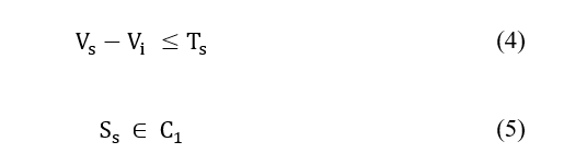
In the end, we used another regional growth to get the whole shape of buildings, and this time used the lightness value (L) from the Lab color space for all the pixels  of the image starting as an initial with the centers  of each superpixel from the final superpixels seed points result take into consideration one condition:

4.2.  Accurate The Final Shape of The Buildings

We can see from the last step that neither the boundaries nor the inside of the building are precisely shaped and filled in figure 3(f); there are still some noises and gaps in it. Therefore, some complementary steps are in need. Firstly, an open morphological operation has been applied to remove the noise and fill the gaps. Then, the buildings’ boundaries were extracted using a simple contour method. The final results are shown in figure 3.

5. Experimental Results

This section includes three subsections: first, the suitable selection of algorithm parameters has been defined. The second subsection presents the classification results with and without texture. And finally, we analyze the results and compare them with other methods. The entire experiment was applied to a dataset from Land Information New Zealand urban aerial image for Auckland with a size of 6400×9600 for each image and 7.5cm ground resolution. The experiment is implemented in Intel 3.2 GHz CPU with 16G memory

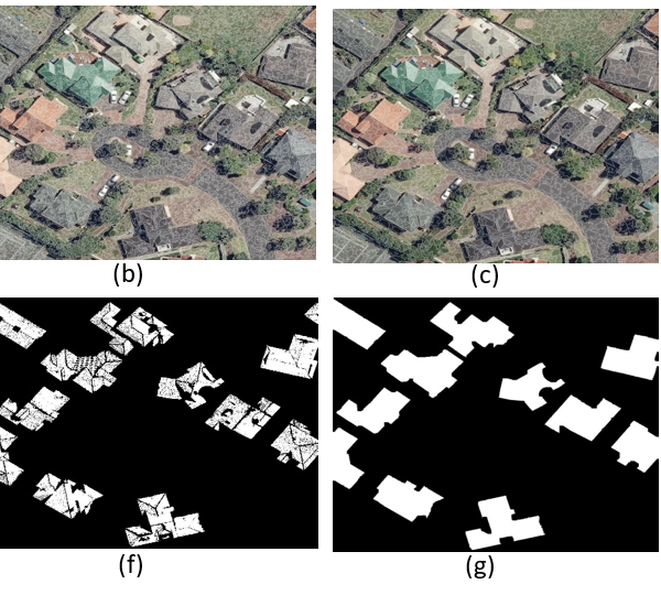
Figure 3. Experimental result of different stages of the algorithm. (a) The original image; (b) Superpixels ; (c) Aggregation Superpixels, (d) classification results, (e) Seed Point Location, (f) after growth (e) Final Shape of The Buildings and (h) The building extraction.

5.1.  Parameters Selection

Three values must be determined ( , , ) where n is the initialized number of the superpixels in the SLIC algorithm,  and are the thresholding of the regional growth in Eqs (4) and (6), respectively. To initial a suitable number n of the superpixels is a two-sided problem. A smaller n leads to fewer calculations and a shorter time in execution. On the other hand, the bigger it is, the better homogeneity we get. That being said, what it depends on is the size and resolution of the image that has been studied. In our test, we use different values of n on a cut from Land Information New Zealand urban aerial image for Auckland with the size of 1286×1249 and 7.5cm ground resolution, and the results reveal that the best value of n is 2500. Therefore, we can define an equation for any image with the exact ground resolution based on that result.

In the same way, for the two thresholding,  and . We can define their values using a sample test and apply the exact values to the rest of the other images.

5.2.  Classification Results

For acceptable outcome classification results, we have to keep an eye on two things. First, as we said before, a proper choice of the initial number of superpixels prevents overlapping groups due to the leak of homogeneity. Second is the selection of training sets for the SVM methods. The more we cover all the possibilities, the better results we get. Under those considerations, figure 4 illustrates the comparison results of the classification with and without adding the texture features. The improvement is much more noticeable when buildings have similar colors to the other classes.

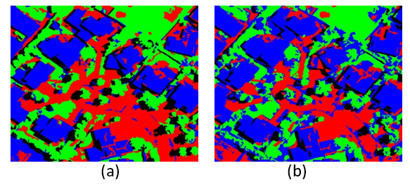
Figure 4. the comparison results of the classification, (a) the classification with the texture features, (b) without adding the texture features, Where the blue represents the buildings, the green the grass and the trees, and the red the road and the sidewalk

5.3.  Building Detection Comparison

In this section, the images selected represent diverse building characteristics such as size, the shape of buildings, and different color combinations of their roofs. Our proposed method has been compared to algorithms presented by method [23], a method [26], and method [15] to give a qualitative comparison with our algorithm. As shown in Figure 5, the images on the first row indicate the original input images where we chose three different images, and the second row illustrates the final building extraction results.

Firstly, the following quantities were defined: TP (true positive), the number of correctly detected buildings, FP (false positive), the number of incorrectly detected buildings, and FN (false negative), the number of undetected buildings. To quantify the accuracy of the building extraction results, we used the detection rate (DR or precision) to measure the degree to which detected buildings indeed are actual buildings. Furthermore, the false-negative rate (FNR) measures the degree of missed detections to the total actual buildings. Meanwhile, the completeness of detection (COMP) is the number of correctly detected buildings without decreasing or increasing their boundaries.

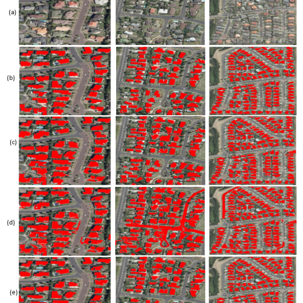
Figure 5: Comparison of building detection results obtained by three different algorithms where (row a) Test images, (row b) The results of the proposed method, (row c) The results of the method [15], (row d) The results of the method [23] and (row e) The results of the method [26]. (Red represents building results).

Table 1: Comparison of the building extraction accuracy of the four algorithms (quantitative analysis of Figure 5).

	Our method	method [23]	method [26]	method [15]
TP	3719	3799	3806	3802
FP	110	749	1083	324
FN	83	56	23	27
DR (%)	97.13	83.53	77.85	92.14
FNR (%)	2.18	1.45	0.6	0.7
COMP	3570	2966	2323	3445
COMP (%)	95.99	78.07	61.03	90.61

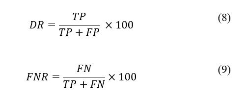
Table 1. shows the comparison results of our approach with existing methods; 50 different sizes of images (3883 buildings) have been taken for testing. Our method has a greater missed detection rate than previous strategies (2.18%). However, it has a more efficient detection rate and completeness (97.13%, 95.99%). That is since those algorithms detected elements other than buildings, such as crossroads, lawns, and parking lots, as a building explaining the high detection rate. Furthermore, because of the background interference and other visual objects, 164 buildings were missed by the proposed method from the total number of buildings. Moreover, the small buildings that were tight distributed may have been excised and integrated as a single building. It might also be that small buildings are harder to detect.

5.4.  Computation Time

Finally, another important consideration for this method is computing time. The proposed methods were implemented in a MATLAB environment; Table 2 contains further information about computation times. Our suggested approach was applied to 50 test images (3,883 buildings); each line in the table represents the elapsed time for every section. The total time is 2146.18 seconds, and the average time is approximately 42.92 seconds.

Furthermore, segmentation takes only 0.34 seconds on average, which is the quickest of all steps. Conversely, the SVM classification takes substantial time, accounting for 92.1 percent of the overall time. Nevertheless, the average time needed to process an image is 42 seconds, much shorter than the approaches presented in [23] and [26].

Through figure 6, We can see that the segmentation images evaluation took 0.06 seconds longer than the feature extraction time of 0.03 seconds in figure 6a and that the time for zoning is less than feature extraction in figure 6b. This is because the regions in the 50 images that were processed had completely different dimensions (2537*3665, 2961*1761, 3465*5601,…etc.) than the area in the tested image (figure. 6B), which has Dimensions (1286*1249).

6. Conclusion

Almost every building detection method has some limitations due to the restrictions that have been applied. This paper presents a pipeline for building detection in 2D urban images by considering two main problems: the color similarity in urban objects and the difference of color shades in building rooftops. The proposed algorithm combines color and texture features to classify the urban image into four classes to solve the first issue. And the reason this is achievable is due to the advantages of using superpixels instead of single normal pixels.

Table 2: The amount of time each section of the proposed building detection

Section	Total Time (s)	Average time (s)	Percentage (%)
Image segmentation	17.02	0.3404	0.8%
Feature extraction	65.83	1.3166	3.1%
Object classification (shadow detection )	1975.58	39.5116	92.1%
The final shape of the building	87.75	1.755	4.1%
Total	2146.18	42.92.36	100%

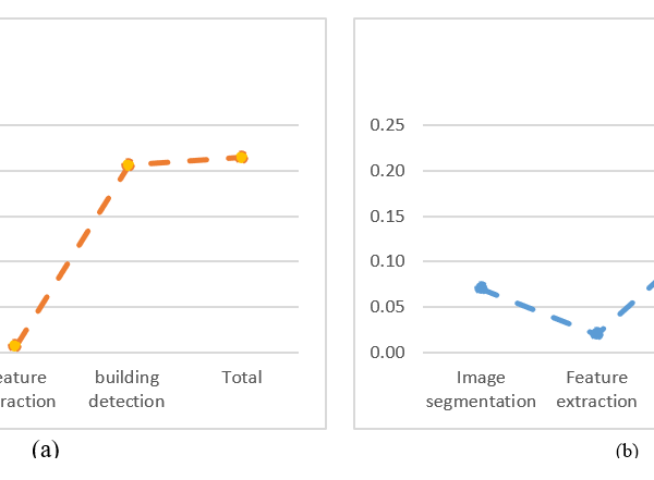
Figure 6. Building detection computational time in sec. Where (a) Total Time of building detection in 50 images and (b) Total Time of building detection in one image.

As for the second one, we use an adaptive regional growth method using only the a and b vectors from the Lab color space with the texture features. After conducting careful analysis, the experimental results revealed a remarkable improvement. Compared to the existing algorithm, the range detection procedure was quick and accurate, and the computing time required to detect the region was also reduced. The automatic detection method used in this work is a reliable methodology that may be used during a catastrophe event. However, some failures are detected in particular cases, like building with different rooftop color parts at once. Therefore, we will target more particular situations to improve detection accuracy in future work.

1. W. Sirko, S. Kashubin, M. Ritter, A. Annkah, Y.S.E. Bouchareb, Y. Dauphin, D. Keysers, M. Neumann, M. Cisse, J. Quinn, “Continental-Scale Building Detection from High Resolution Satellite Imagery,” 1–15, 2021.
2. X. Shen, D. Wang, K. Mao, E. Anagnostou, Y. Hong, “Inundation extent mapping by synthetic aperture radar: A review,” Remote Sensing, 11(7), 1–17, 2019, doi:10.3390/RS11070879.
3. S.L. Ullo, C. Zarro, K. Wojtowicz, G. Meoli, M. Focareta, “Lidar-based system and optical vhr data for building detection and mapping,” Sensors (Switzerland), 20(5), 1–23, 2020, doi:10.3390/s20051285.
4. X. Hou, Y. Bai, Y. Li, C. Shang, Q. Shen, “High-resolution triplet network with dynamic multiscale feature for change detection on satellite images,” ISPRS Journal of Photogrammetry and Remote Sensing, 177(May), 103–115, 2021, doi:10.1016/j.isprsjprs.2021.05.001.
5. U.C. Benz, P. Hofmann, G. Willhauck, I. Lingenfelder, M. Heynen, “Multi-resolution, object-oriented fuzzy analysis of remote sensing data for GIS-ready information,” ISPRS Journal of Photogrammetry and Remote Sensing, 58(3–4), 239–258, 2004, doi:10.1016/j.isprsjprs.2003.10.002.
6. A. Ghandour, A. Jezzini, “Post-War Building Damage Detection,” Proceedings, 2(7), 359, 2018, doi:10.3390/ecrs-2-05172.
7. A. Zhang, X. Liu, A. Gros, T. Tiecke, “Building Detection from Satellite Images on a Global Scale,” (Nips), 2017.
8. K. Karantzalos, N. Paragios, “Automatic model-based building detection from single panchromatic high resolution images,” International Archives of the Photogrammetry. Remote Sensing & Spatial Information Sciences, 37, 225–230, 2008.
9. M. Aamir, Y.F. Pu, Z. Rahman, M. Tahir, H. Naeem, Q. Dai, “A framework for automatic building detection from low-contrast satellite images,” Symmetry, 11(1), 1–19, 2019, doi:10.3390/sym11010003.
10. J.P. Cohen, W. Ding, C. Kuhlman, A. Chen, L. Di, “Rapid building detection using machine learning,” Applied Intelligence, 45(2), 443–457, 2016, doi:10.1007/s10489-016-0762-6.
11. A.M. Cretu, P. Payeur, “Building detection in aerial images based on watershed and visual attention feature descriptors,” Proceedings – 2013 International Conference on Computer and Robot Vision, CRV 2013, 265–272, 2013, doi:10.1109/CRV.2013.8.
12. K. Nogueira, O.A.B. Penatti, J.A. dos Santos, “Towards better exploiting convolutional neural networks for remote sensing scene classification,” Pattern Recognition, 61, 539–556, 2017, doi:10.1016/j.patcog.2016.07.001.
13. Z. Guo, Q. Chen, G. Wu, Y. Xu, R. Shibasaki, X. Shao, “Village building identification based on Ensemble Convolutional Neural Networks,” Sensors (Switzerland), 17(11), 1–22, 2017, doi:10.3390/s17112487.
14. J. Kang, M. Körner, Y. Wang, H. Taubenböck, X.X. Zhu, “Building instance classification using street view images,” ISPRS Journal of Photogrammetry and Remote Sensing, 145, 44–59, 2018, doi:10.1016/j.isprsjprs.2018.02.006.
15. L. Zhang, J. Wu, Y. Fan, H. Gao, Y. Shao, “An Efficient Building Extraction Method from High Spatial Resolution Remote Sensing Images Based on Improved Mask R-CNN,” Sensors, 20(5), 1465, 2020, doi:10.3390/s20051465.
16. N. Shorter, T. Kasparis, “Automatic vegetation identification and building detection from a single nadir aerial image,” Remote Sensing, 1(4), 731–757, 2009, doi:10.3390/rs1040731.
17. M. Ghanea, P. Moallem, M. Momeni, “Automatic building extraction in dense urban areas through GeoEye multispectral imagery,” International Journal of Remote Sensing, 35(13), 5094–5119, 2014, doi:10.1080/01431161.2014.933278.
18. M.S. Nosrati, P. Saeedi, “A combined approach for building detection in satellite imageries using active contours,” Proceedings of the 2009 International Conference on Image Processing, Computer Vision, and Pattern Recognition, IPCV 2009, 2, 1012–1017, 2009.
19. M. Awrangjeb, M. Ravanbakhsh, C.S. Fraser, “Automatic detection of residential buildings using LIDAR data and multispectral imagery,” ISPRS Journal of Photogrammetry and Remote Sensing, 65(5), 457–467, 2010, doi:10.1016/j.isprsjprs.2010.06.001.
20. D. Grigillo, M. Kosmatin Fras, D. Petrovič, “Automatic extraction and building change detection from digital surface model and multispectral orthophoto,” Geodetski Vestnik, 55(01), 011–027, 2011, doi:10.15292/geodetski-vestnik.2011.01.011-027.
21. B. Salehi, Y. Zhang, M. Zhong, V. Dey, “Object-based classification of urban areas using VHR imagery and height points ancillary data,” Remote Sensing, 4(8), 2256–2276, 2012, doi:10.3390/rs4082256.
22. K. Stankov, D.-C. He, “Using the Spectral Similarity Ratio and Morphological Operators for the Detection of Building Locations in Very High Spatial Resolution Images,” Journal of Communication and Computer, 10(March 2013), 309–324, 2013.
23. D. Chen, S. Shang, C. Wu, “Shadow-based Building Detection and Segmentation in High-resolution Remote Sensing Image,” Journal of Multimedia, 9(1), 181–188, 2014, doi:10.4304/jmm.9.1.181-188.
24. J. Wang, X. Yang, X. Qin, X. Ye, Q. Qin, “An efficient approach for automatic rectangular building extraction from very high resolution optical satellite imagery,” IEEE Geoscience and Remote Sensing Letters, 12(3), 487–491, 2015, doi:10.1109/LGRS.2014.2347332.
25. D. Kohli, R. Sliuzas, A. Stein, “Urban slum detection using texture and spatial metrics derived from satellite imagery,” Journal of Spatial Science, 61(2), 405–426, 2016, doi:10.1080/14498596.2016.1138247.
26. Z. Lv, W. Shi, J.A. Benediktsson, X. Ning, “Novel object-based filter for improving land-cover classification of aerial imagery with very high spatial resolution,” Remote Sensing, 8(12), 2016, doi:10.3390/rs8121023.
27. P. Manandhar, Z. Aung, P.R. Marpu, “Segmentation based building detection in high resolution satellite images,” International Geoscience and Remote Sensing Symposium (IGARSS), 2017-July, 3783–3786, 2017, doi:10.1109/IGARSS.2017.8127823.
28. A. Ghandour, A. Jezzini, “Autonomous Building Detection Using Edge Properties and Image Color Invariants,” Buildings, 8(5), 65, 2018, doi:10.3390/buildings8050065.
29. R. Achanta, A. Shaji, K. Smith, A. Lucchi, P. Fua, S. Susstrunk, “SLIC Superpixels Compared to State-of-the-Art Superpixel Methods,” IEEE Trans. on Pat. Anal. and Mach. Intel., 34(1), 1–8, 2012.
30. A. Vadivel, S. Sural, A.K. Majumdar, “An Integrated Color and Intensity Co-occurrence Matrix,” Pattern Recognition Letters, 28(8), 974–983, 2007, doi:10.1016/j.patrec.2007.01.004.
31. B. Khaldi, M.L. Kherfi, “Modified integrative color intensity co-occurrence matrix for texture image representation,” Journal of Electronic Imaging, 25(5), 053007, 2016, doi:10.1117/1.JEI.25.5.053007.

(Click Here)