1. Introduction

In the literature, an agent is defined according to the type of application for which it is designed. In [1]-[3], the authors define an agent is an entity that can be considered as perceiving its environment by means of sensors and acting on this environment by means of effectors.

In this paper, we have chosen to limit the communication between agents to the exchange of knowledge because we are interested in the autonomy of the agent. In [4], [5], the authors specify that the autonomy of the agent is related to its structure: for example, for a cognitive agent that plans to reach its goals, we can talk about autonomy by planning.

For an agent deployed in a MAS, the agent’s autonomy depends on the objective to be achieved, which is:

• Global: this requires cooperation with other agents and limits the agent’s decision-making and behavior and makes the RA algorithm difficult.
• Individual (agent-specific): in this case, the agent can achieve his objectives alone. He does not need to cooperate with other agents. And if it decides to do so, it is to enrich its knowledge base. In this context, the authors of [6] propose characteristics of the autonomous agent:
  • An autonomous agent has its objectives;
  • He can make decisions about his objectives;
  • It can decide autonomously when to adopt the objectives of other agents;
  • He sees cooperation with other agents as a way to enrich his knowledge base to achieve his objectives;

In this context, and concerning our problem and the aspect we want to address, we adopt for our agents the properties proposed by the authors of [6].

The structure of this paper is as follows: after establishing the necessary background and notation in Section 1, we briefly introduce in Section 2 some approaches that use Q-Learning on non-Markovian environments. Then, in Section 3, we give a brief overview of Markov decision process. In Section 4, we give an overview of the mathematical formulas used in reinforcement learning. We then describe our new technique for accelerating the agent learning process based on reinforcement learning in Section 5. Finally, we present some conclusions and suggestions for future work in Section 6.

2. Related Work

In MAS, interaction with the environment, both for perception and action operations and for message sending operations, is synchronous for the agent. On the other hand, the communication between agents remains asynchronous, preventing any assumption on the state of an agent following the sending of a message. The main disadvantage of this domain is that the behavior of an agent will depend on the other agents and thus, we go out of the classical framework of reinforcement learning. This is a problem that has been raised by several researchers:

In [7], the authors show that Q-Learning cannot converge for non-Markovian problems. Indeed, in theory, the convergence of Q-Learning is only possible if the policy used is fixed during the exploration phase of the environment. This policy can be stochastic, but it must be fixed: for a given state, the probability of choosing an action must be constant. This is generally not the case with classical methods. If the exploration policy is fixed, the Q-Learning algorithm converges to the utility estimate of the fixed policy used. This requires the introduction of new techniques in the reinforcement learning algorithm. Several solutions have been proposed:

In [8], the authors present a hybrid Q-learning algorithm named CE-NNR which is springed form the CE-Q learning and NNR Q-learning is presented. The algorithm is then well extended to RoboCup soccer simulation system.

In [9], the authors propose a decentralized progressive reinforcement learning that, based on classical RL (Reinforcement Learning) techniques, allows to endow agents with stochastic reactive behaviors. Indeed, with these stochastic behaviors, the agents will be more efficient in this framework of partial perceptions of the global system.

In [10], the authors first present the principles of multi-agent systems and their contribution to the solution of certain problems. They then propose an algorithm that allows to solve in a distributed way a problem posed globally to the community of agents based on reinforcement learning in the multi-agent framework.

In [11], the authors present a new algorithm for independent agents that allows learning the optimal joint action in games where coordination is difficult. The approach is motivated by the decentralized character of this algorithm which does not require any communication between agents and Q-tables of size independent of the number of agents. Conclusive tests are also performed on repeated cooperative games, as well as on a chase game.

In [12], the authors of this article propose an algorithm called adaptive Q-learning to judge whether the strategy of a particular agent affects the benefit of the corresponding joint action depending on the TD error. In a multi-agent environment, this algorithm makes it possible to adjust the dynamic learning rate between the agents, the coordination of the strategies of the agents can be carried out.

3. Markov Decision Process (MDP)

The problem of learning [13]-[17], like planning, is to control the behavior of an agent. We, therefore, need to model this agent in its environment. The model used considers on the one hand the possible states of the system (=agent + environment) and on the other hand the possible actions of the agent in its environment.

Since the environment is uncertain, it is easy to think of stochastic modeling of the system. The basic tool that will be used for the learning and the general functioning of the agents is the Markov Decision Process (MDP) and its derivatives. This is a class of Markov models, themselves belonging to stochastic processes.

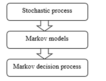
Figure 1: Evolution of the models [18]

The starting idea of a stochastic process is to use as a representation a graph in which the nodes are the possible states of the system and the arcs (oriented and annotated) give the probabilities of passage from one state to another.

3.1.  Stochastic process

Any family of random variables  is called a stochastic process or random process. This means that to any  is associated a random variable taking its values in a numerical set . We denote the process . If T is countable, we say that the process is discrete; if  is an interval, we say that the process is permanent.

3.2.  Markov Model

In the Markov model, at state t, X(t) depends only on the n previous states (memory of the process in a model of order n). At order 1, as it is often the case:

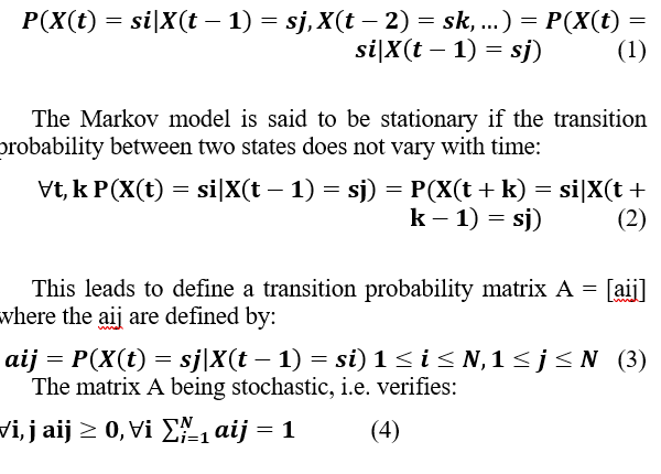
where N is the number of states of the system.

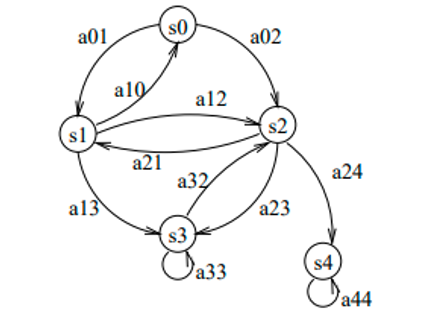
Figure 2: Graph of a Markov model [18].

aij = transition probability of X(i) → X(j).

The agents will be immersed in a world where, starting from a given state, the same action does not always lead to the same state. This may be because the state is only incompletely known (only a partial observation is known), or that simultaneous actions of other agents may take place. Markov models allow modeling such situations.

The different actions performed and the different states encountered will bring any agent again or a cost. The agents must therefore try to act in the best way. Their policies can be diverse depending on whether they consider the more or less long term, different estimates of the expected future gain being possible.

One last point to note is that an agent may not know at the beginning the laws governing its environment. It will then have to learn them more or less directly to improve its chances of winning.

A Markov decision process is a quadruple , where:

• is a set of states called state space,
• is a set of actions called action space (alternatively,   is the set of actions available from state ),
• ( is the probability that action  in state  at time  will lead to state  at time ,
• is the immediate reward (or expected immediate reward) received after the transition from state  to state , due to action

Example:

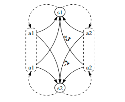
Figure 3: An example of a Markov decision process [18]

3.3.  Use

Starting points: The aim is to maximize the reward in the more or less long term. It is, therefore, necessary to measure the expectation of gain, by taking less and less account of the future (less confidence, thanks to the coefficient: γ ϵ [0, 1]):

Other calculation methods are possible, but only the previous formula will be used in the following.

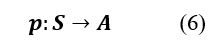
In each state, it will be necessary to determine the optimal action to take. We thus define a policy p:

Values used: the expectation of gain will depend on the chosen policy. We can thus define, for a fixed policy p, the utility of a state:

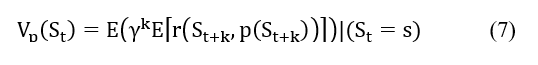
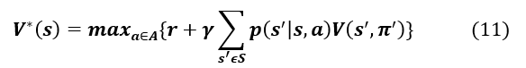
For an optimal policy: V* (s) = Supp Vp(s), the utility of an optimal policy can be written recursively as the Bellman equation:

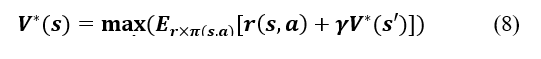
We obtain an optimal deterministic policy by looking for the action for which we obtain this maximum.

In planning, the algorithms called Value Iteration and Policy Iteration allow, starting from any function V, to converge to V* and thus to find an optimal policy.

Another greatness [15], Q (s, a), can be used, obtained from V (s). It will provide the “quality” of the action performed in the state:

3.4.  Others models

From the Markov model, variants are defined which are used in pattern recognition as well as in planning (like MDPs). The general goal is to guess the present or future state of a system. Here are some derived Markovian models:

• HMM: in a Hidden Markov Model, the state of the system is not known. On the other hand, we have an observation that is linked to the states by probabilistic laws. We cannot be sure of a state with a perception of the external world, but a series of perceptions can refine a judgment. This is the main tool for pattern recognition based on Markov models.
• MMDPs (Multiple MDPs) is a variant of MDPs adapted to the case of multi-agent systems, as are DEC-MDPs (decentralized MDPs) and Markov games.
• SMDP: the model, called Semi-Markovian, aims at improving time management, considering that the passage in a state can be of variable duration (according to stochastic laws).

POMDP: this is a mixture of HMMs and MDPs, these Partially Observable MDPs add the idea that an agent has only a partial perception of its environment so that it knows only an observation and not a complete state.

4. Reinforcement learning

4.1.  Principle

Reinforcement learning is one of the most widely used machine learning methods in the world of data science. This technique allows the computer to perform complex tasks on its own. The machine learns from its experiences through a system of penalties or rewards. Reinforcement learning involves an algorithm with great potential: Q-learning. This algorithm focuses on learning a policy that maximizes the total reward. Q-learning focuses on the usefulness of the action to be performed to obtain a reward. The Markov Decision Process is the formal model used for reinforcement learning [19], [20].

A MDP is a tuple  with:

• is a finite set of states,
• is a set of actions,
• , The probability that the agent moves from one state to another is called the transition probability.
• , the reward function.

A very important assumption of reinforcement learning, called the Markov property, is defined on the transition function of the environment states. An environment is Markovian if the transition function to a state depends only on the previous state.

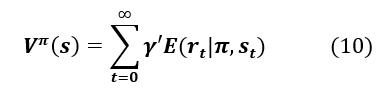
Remember that the agent’s objective is to maximize the total rewards received. In this context, we introduce the notion of a discount coefficient, denoted γ, which allows us to give more importance to nearby rewards rather than to more distant ones. The sum of the rewards is then: , with . In the special case where , the agent maximizes the immediate reward, whereas when , the agent increasingly considers long-term rewards.  represents the duration of an episode that corresponds to a sub-sequence of interaction between the agent and the environment.

The value function  represents the quality of state s in terms of the expected reward from following policy π. Formally, this value function is defined by:

Similarly, we define the value function  as the expectation of the reward if the agent prefers the action in state s and follows the policy π thereafter. Finding a solution to a reinforcement learning problem comes down to finding a policy that maximizes the sum of long-run rewards. Bellman’s optimal equation for  describes the fact that the optimal value of a state is equal to the expected reward for the best action in that state. More formally:

The relationship between  and  is represented by the equation . From the optimal value function , we define the optimal policy as .  If the dynamics of the system is known, it is possible to solve the problem using dynamic programming to find the optimal policy. In cases where the dynamics of the system are not known, one must either use estimation or use a set of methods, called time-difference learning (TD-Learning), which are able to evaluate the optimal policy through the experiences generated by an interaction with the system. One of the main algorithms for computing the optimal policy, Q-Learning, uses the Q-value function. This algorithm works by interacting with the environment in the following way: in each episode, the agent chooses an action  based on a policy  derived from the current values of . It executes action , receives the reward, and observes the next state. Then it updates the values of  by the formula:

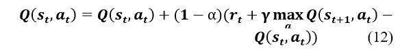
where  is the immediate reward,  is the new state,  is the learning rate. The convergence of this algorithm to the optimal value function has been demonstrated in [21]. The choice of action at each step is made using exploration functions. Among these methods we can mention the voracious, e-voracious and softmax approach which choose an action at random according to a certain probability. For a more exhaustive description of exploration functions, one can refer to[8], [22].

Hence the algorithm:

Algorithm 1: Q-Learning
Initialize Q0 (s,a) arbitrarily;
Choose a starting point s0;
while the policy is not good enough {
	Choose at as a function of Qt (St,.);
	In return: st+1 and rt
	;
}

The coefficient α should then be adjusted to gradually fix the learned policy. γ allows for its part to modulate the importance of expected future rewards.

4.2.  Implementation

Two factors must be defined to apply the Q-learning algorithm: first, the learning factor , which determines to what extent the newly calculated information outperforms the old one. The latter must be between 0 and 1, and decrease towards 0 because if , the agent learns nothing. On the other hand, if , the agent always ignores everything it has learned and will only consider the most recent information. Second, the discount factor   determines the magnitude of future rewards. A factor of 0 would make the agent myopic considering only current rewards, while a factor close to 1 would also imply more distant rewards. In our approach, we chose:  and .

It remains to choose the actions to be carried out according to the knowledge acquired.

5. Proposed approach

In our proposed approach, the agent can achieve its goals alone. The cooperation with other agents is limited to the exchange of Qtable learning tables to enrich its knowledge base. To do so, after each new exploration, the agent has to communicate its learning table Qtable to the other agents, and the latter have to build their knowledge bases taking into account this Qtable. And each agent that wants to explore the environment again must use its knowledge base, i.e. the values of the last Qtable communicated by the environment, as initial values of its Qtable. This allows the agent to gain a large exploration step and subsequently accelerate the speed of the learning process.

5.1.  The class diagram

In the class diagram shown in Figure 4, agents are autonomous entities hosted in a graphical environment. Each node of this graph represents a state, and the links between these nodes represent the transitions between these states. There are three types of states in this environment: with penalties, without penalties and obstacles.

In this case, reinforcement learning is applied as follows:

• The transition that allows access to the final state (the goal) is represented by a reward equal to 100.
• The transition that leads to an obstacle is represented by a reward equal to -1.
• The transition that allows access to other states: -10 for states with penalties and 0 for normal states.

The agent must maximize its rewards which allows it to reach the optimal path to the final state.

In the learning phase, the experience of agents who have already explored the environment can be used to improve the speed of the adaptation and learning process of other agents. Indeed, before the start of learning, the function is initialized by the Q values of the last agent having explored the environment. After learning, the agent shares the new Q-values with the other agents in order to use them as initialized values for a new exploration.

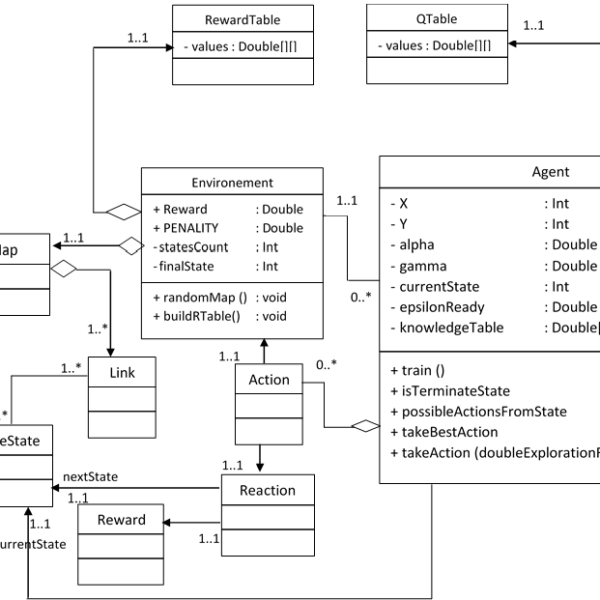
Figure 4: The class diagram of our approach

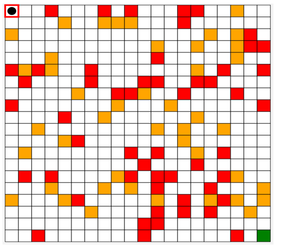
Figure 5: An example of the environment generated in the simulator we have developed.

5.2.  Experiment

We have chosen a maze-like environment to test our model. The number of rows and the number of columns of this environment are chosen randomly using the following function:

Algorithm 2:
this.map=new char[rows][cols];
for (int i = 0; i < rows; i++){
for (int j = 0; j < cols; j++) {
	double rnd=Math.random();
	if (rnd<0.75) this.map[i][j]=’0′;
	else{ this.map[i][j] = (Math.random() > 0.5) ? ‘P’ : ‘W’;}
} }

To test our application, we choose our environment as a maze where 75% of the cells represent normal states and the rest represent obstacle and penalty states (see Figure 5).

To build the rewards table, the application calls the buildRewardTable function as follows:

Algorithm 3:
public void buildRTable(){
	for (int k = 0; k < statesCount; k++) {
		int row=k/gridWidth;
		int col=k%gridWidth;
		for (int s = 0; s < statesCount; s++) {
			System.out.println(s+”->”+k);
			R[k][s]=-1; }
		if (map[row][col]!=’F’){
			for(int[] d :directions){
				int c=col+d[1];
				int r=row+d[0];
				if ((c>=0 && c<gridWidth)&&(r>=0 && r<gridHeight)){
					int st=r*gridWidth+c;
					if (map[r][c]==’0′)
						R[k][st]=0;
					else if (map[r][c]==’W’)
							R[k][st]=-1;
						else if (map[r][c]==’F’)
								R[k][st]=EnvGrid.REWARD;
							else if (map[r][c]==’P’)
									R[k][st]=EnvGrid.PENALTY;
				}
			}
		}
	} }

The learning of the agents is described by the code below; it allows the construction of the learning table Qtable. The values of this table are computed as follows:

• The agent tries at each learning period to find a solution to achieve the objective.
• Each time, the agent repeats random movements between the states by performing the possible actions.
• For each transition, the value of the Qtable is calculated.

Algorithm 4:
public void train(){
	Random random=new Random();
	for (int i = 0; i <1000 ; i++) {
		this.currentStat=random.nextInt(envGrid.statesCount);
		while (!isTerminalState()){
			int[]
			possibleActionsFromState=possibleActionsFromState(currentStat);
			int index=random.nextInt(possibleActionsFromState.length);
			int nextState=possibleActionsFromState[index];
			double q=Q[currentStat][nextState];
			double maxQNextState=maxQ(nextState);
			double r=envGrid.R[currentStat][nextState];
			double value=q+alpha*(r+gamma*maxQNextState-q);
			Q[currentStat][nextState]=value;
			currentStat=nextState;
		}
	}}
public int[] possibleActionsFromState(int state){
		List<Integer> states=new ArrayList<>();
		for (int i = 0; i <envGrid.statesCount ; i++) {
			if(envGrid.R[state][i]!=-1) states.add(i);
		}
		return states.stream().mapToInt(i->i).toArray();
	}

• Result

The graph in Figure 6 shows the evolution of an agent’s learning process that started with a randomly defined knowledge base and no experience:

This agent must communicate his experience (his Qtable) to the other agents. The latter will use it as an initial Qtable for new exploration.

The graph in figure 7 shows the evolution of the learning process of an agent who used the experience of another agent who had already explored the environment, i.e. he initially used the latter’s Qtable as a knowledge base.

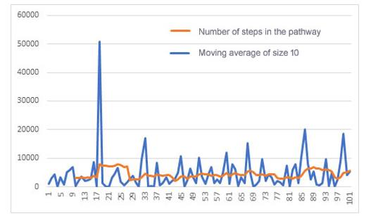
Figure 6: Number of learning path states for the first 100 epochs of an agent with an empty knowledge base (initial Qtable).

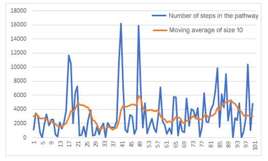
Figure 7:Number of learning path states for the first 100 epochs of an agent

Figure 8 show the paths taken by the last agent for three trials at different initial positions. We see that the agent correctly takes the optimal path with sometimes the preference to cross a penalty point in a minimum number of moves.

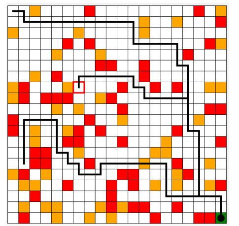
Figure 8: Execution.

6. Conclusion and Future Work

In this paper, we have proposed an approach based on reinforcement learning to solve the problem of cooperation between agents in multi-agent systems. To do so, we proposed in the agent structure that cooperation is limited to the exchange of new knowledge. Indeed, an agent who has just explored the environment must send the new knowledge collected to the other agents, and the latter use this knowledge for new exploration. To validate our method, we chose to evaluate it in a grid environment. Agents must exchange their tables (Qtables) to facilitate better exploration. According to the results, the experiences of the agents that have already explored the environment help to accelerate the reinforcement learning process in MAS. This allows the agent to take an important exploration step and then reach its goal faster.

Ensuring communication between agents in different environments is the goal of our future work. Ontologies can meet this need, that is to enrich the knowledge base of agents with new knowledge provided by other environments. And this requires migrating to other environments, our idea is to use a mobile agent that can migrate to other environments to collect new knowledge and share it with other agents. The mobile agent receives rewards in return.

1. N. Carlési, F. Michel, B. Jouvencel, J. Ferber, “Generic architecture for multi-AUV cooperation based on a multi-agent reactive organizational approach,” IEEE International Conference on Intelligent Robots and Systems, 5041–5047, 2011, doi:10.1109/IROS.2011.6048686.
2. P. Ciancarini, M. Wooldridge, “Agent-oriented software engineering,” Proceedings – International Conference on Software Engineering, 816–817, 2000.
3. Z. Papp, H.J. Hoeve, “Multi-agent based modeling and execution framework for complex simulation, control and measuring tasks,” Conference Record – IEEE Instrumentation and Measurement Technology Conference, 3(section 2), 1561–1566, 2000, doi:10.1109/imtc.2000.848734.
4. X. Yang, Z. Feng, G. Xu, “An active model of agent mind: The model of agent’s lived experience,” Proceedings – 2009 International Conference on Information Engineering and Computer Science, ICIECS 2009, 3–5, 2009, doi:10.1109/ICIECS.2009.5364300.
5. A. Kumar, A. Tayal, S.R.K. Kumar, B.S. Bindhumadhava, “Multi-Agent autonomic architecture based agent-Web services,” Proceedings of the 2008 16th International Conference on Advanced Computing and Communications, ADCOM 2008, 329–333, 2008, doi:10.1109/ADCOM.2008.4760469.
6. M. Huang, P.E. Caines, R.P. Malhamé, “A locality generalization of the NCE (Mean Field) principle: Agent specific cost interactions,” Proceedings of the IEEE Conference on Decision and Control, 5539–5544, 2008, doi:10.1109/CDC.2008.4738976.
7. S. Filippi, O. Cappé, A. Garivier, “Optimally sensing a single channel without prior information: The Tiling Algorithm and regret bounds,” IEEE Journal on Selected Topics in Signal Processing, 5(1), 68–76, 2011, doi:10.1109/JSTSP.2010.2058091.
8. W. Chen, J. Guo, X. Li, J. Wang, “Hybrid Q-learning algorithm about cooperation in MAS,” 2009 Chinese Control and Decision Conference, CCDC 2009, 3943–3947, 2009, doi:10.1109/CCDC.2009.5191990.
9. Y. Xu, W. Zhang, W. Liu, F. Ferrese, “Multiagent-based reinforcement learning for optimal reactive power dispatch,” IEEE Transactions on Systems, Man and Cybernetics Part C: Applications and Reviews, 42(6), 1742–1751, 2012, doi:10.1109/TSMCC.2012.2218596.
10. P. Zhou, H. Shen, “Multi-agent cooperation by reinforcement learning with teammate modeling and reward allotment,” Proceedings – 2011 8th International Conference on Fuzzy Systems and Knowledge Discovery, FSKD 2011, 2(4), 1316–1319, 2011, doi:10.1109/FSKD.2011.6019729.
11. L. Matignon, G.J. Laurent, N. Le Fort-Piat, “Hysteretic Q-Learning : An algorithm for decentralized reinforcement learning in cooperative multi-agent teams,” IEEE International Conference on Intelligent Robots and Systems, 64–69, 2007, doi:10.1109/IROS.2007.4399095.
12. M.L. Li, S. Chen, J. Chen, “Adaptive Learning: A New Decentralized Reinforcement Learning Approach for Cooperative Multiagent Systems,” IEEE Access, 8, 99404–99421, 2020, doi:10.1109/ACCESS.2020.2997899.
13. R. Bellman, The Theory of Dynamic Programming, Bulletin of the American Mathematical Society, 60(6), 503–515, 1954, doi:10.1090/S0002-9904-1954-09848-8.
14. D.P. Bertsekas, C.C. White, “Dynamic Programming and Stochastic Control,” IEEE Transactions on Systems, Man, and Cybernetics, 7(10), 758–759, 2008, doi:10.1109/tsmc.1977.4309612.
15. R. ABellman R., and Kalaba, “Dynamic Programming and Modem Control Theory,” Academic Press, New York; 1965., 4, 1–23, 2016.
16. S.E. Dreyfus, “Dynamic Programming and the Calculus of Variations,” Academic Press, New York, 1965.
17. D.T. Greenwood, “Principles of Dynamics,” Prentice-Hall, Englewood Cliffs, N. J., 1991.
18. G. Mongillo, H. Shteingart, Y. Loewenstein, “The misbehavior of reinforcement learning,” Proceedings of the IEEE, 102(4), 528–541, 2014, doi:10.1109/JPROC.2014.2307022.
19. A.O. Esogbue, “Fuzzy dynamic programming: Theory and applications to decision and control,” Annual Conference of the North American Fuzzy Information Processing Society – NAFIPS, 18–22, 1999, doi:10.1109/nafips.1999.781644.
20. E.F. Morales, J.H. Zaragoza, “An introduction to reinforcement learning,” Decision Theory Models for Applications in Artificial Intelligence: Concepts and Solutions, 63–80, 2011, doi:10.4018/978-1-60960-165-2.ch004.
21. F. Khenak, “V-learning,” 2010 International Conference on Computer Information Systems and Industrial Management Applications, CISIM 2010, 292, 228–232, 2010, doi:10.1109/CISIM.2010.5643660.
22. J. Fiala, F.H. Guenther, “Handbook of intelligent control: Neural, fuzzy, and adaptive approaches,” Neural Networks, 7(5), 851–852, 1994, doi:10.1016/0893-6080(94)90107-4.

(Click Here)