1. Introduction

Modeling physical phenomenons is an increasing topic in science and engineering projects. A very accurate model is not only a validation of theory, but a significantly affordable option for test performing without put in jeopardy any actual equipment or material. Hence, the necessity for accurate models provides a research line leading to expand the state of art of current techniques. Alongside, in order to incorporate realistic behavior and obtain valid simulation results, software algorithms are more powerful and faster. However, the more complicated is the model, the more computational work is required. The need of accurate model must be compared with the processing power available for the project and, in most of the cases, the researches has limited resources. The mathematical model used to describe the behavior of thermal conduction is the Fourier heat equation, a second order-partial-differential equation that includes the time and space behavior of the temperature in a solid body. The solution of this equation has been widely studied in different papers,  and it has become in a handy useful tool for introduction in partial-differential equations theory. Tough the solution is known, interpretation and programing in computational simulator may not be as simple, due to the solution is described in literature as a Fourier series [1] and different approaches to deal with the solution [2], [3]. In order to obtain a simplified version of this model, a discrete Fourier equation is developed in [4]. The space discrete model becomes then in a linear system of ordinary differential equations, with the temperature in each segment as the dependent variables and time as only independent variable. This new model fits to results given by the Fourier series solution, with an error estimation related to the physical parameter involved in Fourier equation, density, specific heat and thermal conductivity. These three parameters are non-constant, even two objects of the same material, but they are easily obtained with experimental data. Density is the simplest of them all, due to density is the ratio of mass and volume of the object. Specific heat is more sophisticated, but with a simple temperature test, the value can be calculated as shown in [5], [6] and [7] . A similar experiment may be applied for thermal conductivity, obtaining the average thermal conductivity of the object. Using the space-discrete Fourier equation and a experiment shown in [8] to calculate the thermal conductivity in every segment of the object, the resulting values provides a description of the thermal conductivity along the object. Furthermore, using multiple measure points provides multiple conductivity values, and using a Gauss-Markov estimator, the thermal conductivity in any space position of the bar is calculated. Moreover, the calculation are supposed correct, but there is an uncertainty related to each calculation. In order to describe the error propagation in the calculation of thermal conductivity, an uncertainty analysis is conduced, leading to a range of values in which the correct thermal conductivities are bounded. The work is presented in the following order. Section 2 provides a fundamentals review including the mathematical involved, such as the Fourier equation, its space-continuous and space discrete solution and comparison, and the concept of thermal parameters. Section 3 presents the thermal conductivity estimation using simulated data and the methodology of the experiment, including varying punctual thermal conductivity. In Section 4 it is presented an uncertainty analysis, and the estimation of propagation error. Finally, in section 5, the conclusions and future work are presented.

2 Fundamentals

In this section, the fundamentals and theory applied in the present work are introduced. The general concepts and descriptions are focused referring to the present article. For further information the reader is referred to the selected bibliography included at the document closure.

2.1     Fourier heat equation

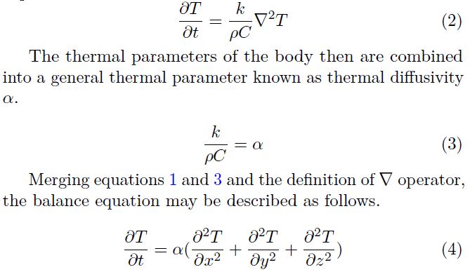
The thermal transference in a solid rigid body is represented by the Fourier heat equation, a partial-differential equation developed by Fourier at lately 19th century. The equation balances the thermal energy provided by the temperature evolution in time and the temperature evolution in space. This balance is represented in equation 1. Fourier heat equation is aim of several studies in differential equations solutions. Some of this works provide an analytical solution using Fourier series, but there are numerical solutions also. The solution of Fourier equation may be obtained in analytical form using Fourier series [1], applying Fourier analysis [2] or using semi-analytical approaches [3].

With

• ρ the body density in ^Kg_m3
• C the body specific heat in _Kg^J_oC
• T the body temperature as a function T(t,x,y,z)
• k the body thermal conductivity in _m^W_oC
• ∇ the operator defined as ∇ = (_∂x^∂ _∂y^∂ _∂z^∂ )

The right side of equation 1 contains the Laplacian of temperature. Solving for, the right side becomes in the expression below.

2.2 Continuous solution of 1 space-dimensional Fourier heat equation

The solution presented is based on traditional analytic approach performed in reference [1]. In order to simplify the mathematical involved in this work, the solution of the Fourier heat equation is shown in the 1 dimensional case, thus, the temperature function has only two independent variables, time t and dimension x. Therefore, the Fourier equation in this case is represented en equation 5. For this solution method, the thermal parameter α is considered constant for both of the independent variables.

Find a numerical solution is an accurate path to avoid the mathematical complexity shown in the continuous solution above. Furthermore, the solution in 3 dimension is more complex and requires larger calculations. For the Fourier equation, one of the most applied numerical methods is the differential discretization proposed by Euler. Using a discrete-space approximation leads to result similar to finite volumes technique, as seen in reference [9].

To achieve a space discretization, the finite differences method is applied [10].

Definition 1 Let f : R → R be a continuous and differentiable function. The differential f⁰ at the point x = a is approximated by the following expression

with b a value sufficiently close to a.

Previous definition is applied for non-even partitions. For the discrete method, even partitions are required, leading to following definition.

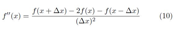
Definition 2 Let f : R → R be a continuous and differentiable function. Assume the domain of the function is partitioned in sufficiently small intervals with length ∆x. The differential f⁰(x) is given by

Using definition 2, the first order differential of Fourier heat equation becomes discrete. For the second order differentials, the same algorithm may be used for the first order differential.

Definition 3 Let f : R → R be a continuous and at least twice differentiable function. Assume the domain of the function is partitioned in sufficiently small intervals with lenght

∆x. The second order differential f⁰⁰(x) is given by

However, the second order differentials in Fourier equation are partial. Moreover, the function T is not defined from real numbers to real numbers. A more accurate interpretation of the second order partial differentials is given in definition 4.

Definition 4 Let f : Rⁿ → R be a continuous and at least twice differentiable function. Assume the domain of every independent variable x_i of the function is partitioned in sufficiently small intervals with lenght ∆x_i. The second order partial differential  of the variable x_i is given by equation 11.

Using definitions 2 and 4, both sides of the Fourier equation are expressed in discrete form in equations 12-14 and 15 respectively. Remembering that temperature T(t,x,y,z) is function defined from R⁴ → R.

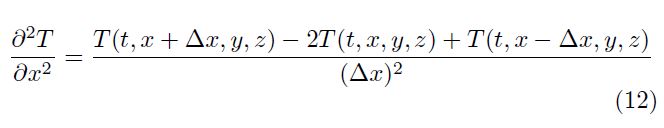
In order to compute the differentials appearing in equations

12-15, the rigid body is then meshed in a set of stationary points, such in time as in space.

Definition 5 A node in a rigid body is a space position with coordinates (x,y,z). The temperature of each node in a time instant t is given by T(t,x,y,z). The distance between two adjacent nodes in space variable x is ∆X. Same description for distance in space variable y and z. The value ∆t is known

as the sampling period.

To ignore the ∆ values, the nodes are numerated and indexed for each of the four variables.

Definition 6 The temperature in the node (l,i,j,k) is the result of value the function

T(l ∗ ∆t,i ∗ ∆x,j ∗ ∆y,k ∗ ∆z),

and it is identified by the indexing T_(i,j,k,l)

Rewriting the equations 12-15 using definition 6, the following expressions are obtained.

 Equations 16-19 are expressions depending only of node index and the constant ∆ values. Using this expressions,  ∂t _l,i,j,k  ∆t the Fourier heat partial-differential equation becomes in an ordinary linear equation, as shown in equation 24. In order to defined the parameters ∆t,∆x,∆y and ∆z, the sampling theorem postulated by Nyquist and Shanon is applied.2.3     Sampling considerations

Theorem 7 (Sampling theorem [11]) Let s(t) a continuous time function and F(s(t)) its Fourier transform. Assume that F is bandwidth limited by the frequency f_c. The function s(t) can be reconstructed if and only if the sampling frequency f_s satisfy

                                                  f_s > 2f_c                                                          (20)

For a system response, the frequency f_c is associated to the slowest pole. The value of the slowest pole of the system matches the value of f_c in rad/s. In a thermal system, the value of poles may be extremely near to 0, due to the slow temperature variation. Sampling period T_s is defined as the inverse of sampling frequency f_s. Therefore, sampling periods in thermal system can be significantly extended in comparison to other dynamical systems, such as electrical. Time sampling periods for thermal systems are defined in minutes.

For the space sampling, meaning, the distance between the nodes, a slight variation of sampling theorem is used.

Lemma 8 Let R(x) be a one dimensional space function with domiain [0,l] and F(R(x)) its space Fourier transform. F domain is upper bounded by ¹_l . Signal R can be reconstructed at 99.9% of accuracy if the sample nodes are placed with a distance d_s

l    d_s =       10                                      (21)

Using these approach, the minimal distance between nodes along x axis can be calculated as

lx   ∆x =        10                                    (22)

with l_x the length of the body along x axis. Hence, the

minimal required nodes per axis is eleven.

Using equation 24 and solving for T_(l+1,i,j,k), it is possible to calculate the temperature for a fixed node, using information of adjacent nodes in the previous sample.

2.4        Space-state model for temperature distribution

As shown in previous subsection, the discrete approach of Fourier equation leads to a numerical solution, and it is widely used in discrete estimations. However, in order to propose a continuous control algorithm as well as a continuous state observer a continuous space-state model is required. For the continuous model the following considerations are imperative

• Every state of the model represents the temperature of a particular node in the rigid body.
• The nodes on the body surface experiment conduction and convection at the same time, so the equations for these nodes are different from the rest.
• Fourier equation defines the system natural response, no input is applied.
• The number of nodes is previously calculated and exposed in subsection 3.
• Only space discretization is being considered, time remains continuous.

Following the previous considerations, the time differentials of equation 24 remains continuous. The l index is ignored, hence the equations is rewritten as seen on equation

The symbol T^˙_(i,j,k) is used as differential representation. Using equation ??, the continuous differential of each node temperature is calculated as a linear combination of the rest of node temperatures, in particular only the adjacent nodes contribute. Therefore, the temperatures are presented in a space-state representation.

2.5     One-dimensional state-space representation

In order to explain the model in more detail, the first approach is made for only one space dimension heat flow, considering n nodes evenly distributed.

Excluding the border nodes, the remaining n−2 nodes are represented by equation ??, but ignoring the j and k indexes

and the y and z respective differentials. Hence

In matrix condensed form, the space state is represented as seen in equation 31.

For the border nodes, thermal energy interaction is defined by two independent processes, conduction and convection. In convection process, Newton law is applied.

Moreover, a border node has only one adjacent node in the one-dimensional approach. Hence, the Fourier equation is reduced. dt ρc

The complete model obtained from Fourier and Newton equation is presented in equation 32. This expression represents a continuous space-state model for the temperature of the nodes in the body. Though the model is no linear, due to the appearance of environmental temperature, the linear system decomposition matches with the n × n matrix in equation 32. Using these matrix, the stability of the system can be analyzed obtaining the eigenvalues. Moreover, the model can be extended, including external energy inputs and output temperature sensors, leading to a controllability and observability analysis.

2.6     Thermal conductivity

Thermal conductivity is one of the three thermodynamical parameters involved in Fourier heat equation (eq. 1), and there are previous analysis remarking the heat coefficients, as in [12]. Thermal conductivity, definition and formulas are introduced in this subsection.

Definition 9 Thermal conductivity k is the ratio of heat per length unit and temperature variation.

With

• k thermal conductivity in _m^W₂
• Q the heat flow
• L the body length
• A the traversal section area
• ∆T the temperature variation

A comparative method for calculating thermal conductivity is shown in [8]. The comparison requires a material with known thermal conductivity k₂ coupled to an unknown thermal conductivity material k₁. Considering no heat loss, heat flow remains constant in steady state. Thermal conductivity k₁ can be calculated using equation 34.

2.7     Non-homogeneous thermal conductivity

Furthermore in this section, lets consider the thermal conductivity of the bar modeled by equation 32 is not constant. Hence, the case a non-homogeneous thermal conductivity is analyzed. Thermal conductivity, as explained in section 2.6, represents the ratio of heat flow along a determinate length and the temperature variation. Then, thermal conductivity is defined in length intervals. Considering the nodes defined in definition 5, the segment between every couple of adjacent nodes may have a different thermal conductivity. This distribution is illustrated in figure 1. Considering non-homogeneous thermal conductivity, the expression 3 can not be used as a simplification for thermal parameters. In order to obtain a model that considers non-homogeneous thermal conductivity, other assumption is applied. Using equation 25, the epxression is rewritten to appreciate the different thermal conductivities, in equation 35 consider K_m as the total thermal conductivity of the two segments. Then, in equation 36, the nodes are isolated from every segment, hence thermal conductivity for every segment is used. All the terminus are regrouped to obtain equation 37.

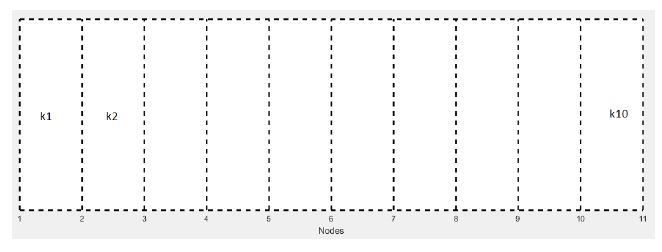Figure 1: Rigid body with non-homogeneous thermal conductivity

For the border nodes, a similar analysis is applied. Considering that in border nodes the conduction is only present in one side, the expression for border nodes is presented in equation 38.

3 Thermal conductivity estimation

This section presents a method for thermal conductivity characterization in a solid rigid body. The experiment is based in the technique of concentric cut bars shown in [8] for homogeneous thermal conductivity. Merging the described experiment with the node representation of a solid body introduced in section 2.7, a method to determinate thermal conductivity per node in real time. The experiment presented in [8] consist of two different materials aligned in concentrically form. A heat source is placed in an edge of material A. This material has a known thermal conductivity. As the heat is transferred along the materials by conduction, the temperature at the edge of the materials is measured. Three points are measured, the edge of material A (nearest from heat source), the contact point of two materials and edge of material B (farthest to

heat source). Only one directional heat flow is allowed, so the materials are isolated. Once thermal equilibrium point is achieved, the values of temperature are used in equation 40 to calculate thermal conductivity of material B. Thermal conductivity can be calculated using the equation 39, as seen on section 2.6

Lets consider one dimensional heat flow, an isolated rigid body composed of two different materials, with respectively thermal conductivities k_a and k_b and a heat source located in one of the body’s edges. Using equation 34 with the steady state temperature measurements and considering the cross area is equal, thermal conductivity k_b of an unkown material is calculated with equation 40, with ∆T_a the temperature difference between the borders of material a, L_a the length of material a and ∆T_b the temperature difference between the borders of material b, L_b the length of material b.

Knowing the nominal thermal conductivity in material b, and using the approach given by the node representation defined in 5 and equation 36, in steady state the heat flow in each of the nodes is equal to 0. This fact is corroborated for the model presented in equation 32, due to equilibrium point of the space state system is calculated when the differentials of each node temperature is zero. T^˙_i = 0. Hence, using Fourier heat equation represented in the form of equation 25

3.1      Simulated thermal conductivity estimation

The procedure above is used to estimate thermal conductivity for simulated data. Using temperature derived from the model described in section 2.7. For the simulation is performed in the complement Simulink of Matlab. For the simulation the following values are considered.

• k₁= 220 (Aluminum)
• L=0.5 m
• ∆x = 0.05m
• ρ = 2675 mkg3
• c= 897 kgJoC

The aluminum bar is represented in nodes and the space state equation given by 32 is programed in simulink using a value of ∆x = 0.05m, and the temperature values for each node are obtained. The parameter of thermal conductivity in the segment between nodes six and seven is set to a value of 187, the rest of the nodes thermal conductivity are set to 220. Using the temperature values for each node, thermal conductivity of each segment is the calculate using equation 44, considering the nominal thermal conductivity of aluminum for the initial thermal conductivity. The results for thermal conductivities in each segment are presented in table 1.

Table 1: Thermal conductivity of each segment in the simulated aluminum bar

Segment	Left temperature	Right temperature	k
	(◦C)	(◦C)
1	45.1478	44.1361	220
2	44.1361	43.1244	220
3	43.1244	42.1126	220
4	42.1126	41.1009	220
5	41.1009	40.0892	220
6	40.0892	38.8991	187.03
7	38.8991	37.8874	220
8	37.8874	36.8756	220
9	36.8756	35.8639	220
10	35.8639	34.8522	220

The temperature in the nodes are presented in figure 3. Results of table 1 in graphic form are observed in figure 2, the variation of temperature along the bar is small, hence the slope of the graphic may not vary even the thermal conductivity is different in the red segment. The method not only provides an accurate value of thermal conductivity, it also isolates the only thermal conductivity variation as if it was related to another material incrusted in segment 5. Figure 4 shows the evolution of segment 5 thermal conductivity along time.

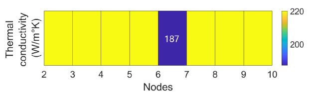Figure 2: Thermal conductivity along the bar in steady state

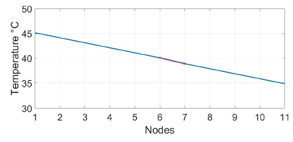Figure 3: Temperature along the bar in steady state

Figure 4: Thermal conductivity of segment 5

4 Uncertainty analysis

The results presented in section 3 are consistent with the calculation of thermal conductivity for the anomaly detected in the simulated bar. Since this is a simulation, no external consideration has been made. However, the data obtained for the temperature measurements are limited by the uncertainty of the sensor used for this purpose. Moreover, with each calculation a new thermal conductivity is obtained, and this new value becomes an uncertainty source for the new calculation, leading to a error propagation. In this section, an analysis of uncertainty and error propagation is presented in order to obtain a range of values to bound the thermal conductivity values obtained using the method presented in section 3.

Definition 10 (Uncertainty) Uncertainty is a parameter, associated with the result of a measurement, that characterizes the dispersion of the values that could reasonably be attributed to the measurand [13]

Let y be the final measurement of a procedure and variables x₁,x₂,··· ,x_n the uncertainty sources. Assume all the variable x_i are not correlated. Then, y can be expressed as a function of variables x_i as seen in equation 46.

                                          y = f(x₁,x₂,··· ,x_n)                                    (46)

The combined uncertainty U_c(y) for the measurement y is calculated by equation 47.

With u(x_i) the corresponding uncertainty of each x_i variable.

The term  is known as the sensibility coefficient for

i variable x_i.

In section 3, equation 44 is used to calculate a thermal conductivity using temperature measurement points. Matching this with equation 46, leads to a function to calculate thermal conductivity k_i+1 using as inputs: thermal conductivity k_i and temperatures T_i−1,T_i,T_i+1, as seen on equation 48

 

Considering the measurements are made with an extremely accurate temperature meter, the uncertainty related to temperature measurement in each node is set as u(T_k) = 0.05^oC. Hence, for the first segment the thermal conductivity is taken as nominal, then k₀ = 220. Using equations 53-56, and information in table 1, the sensibility coefficients for output k₁ are calculated next.

Thus, the interval of values for thermal conductivity are [193.43 246.57]. Even if the range is quite near the expected value, the iterative method to calculate the rest of thermal conductivities in the bar leads to an error propagation, increasing the uncertainty value for every segment of the bar. In table 2 the values of uncertainty for each thermal conductivity are shown.

Table 2: Uncertainty for each thermal conductivity

Segment	Sensibility coefficients	Uc(ki−1)	Uc(ki)
	(ki−1,Ti−1,TiTi+1)	All u(T) = 0.05
k1	(1, 217, 434, 217)	0	26.57
k2	(0.99,217 ,434 ,217)	26.57	37.66
k3	(1,217 ,434 ,217)	37.66	46.13
k4	(1,217 ,434 ,217)	46.13	53.26
k5	(0.85,217 ,434 ,217)	53.26	52.53
k6	(1.17,157 ,369 ,184)	52.53	65.63
k7	(1,217 ,434 ,217)	65.63	70.82
k8	(1,217 ,434 ,217)	70.82	75.67
k9	(1,217 ,434 ,217)	75.67	80.22
k10	(1,217 ,434 ,217)	80.22	84.52

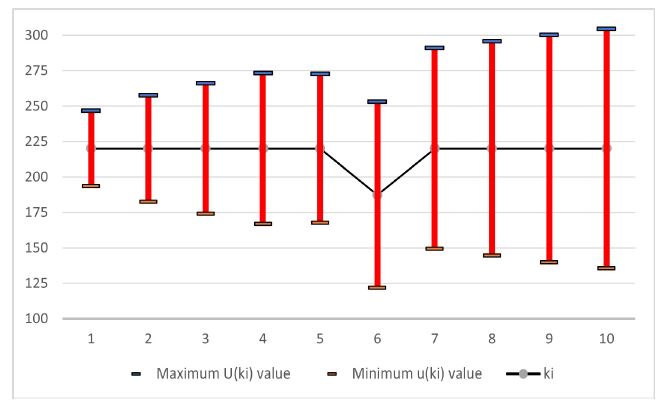Figure 5: Thermal conductivity uncertainty along the bar in steady state

Table 2 shows that the uncertainty in the segment 10 of the bar is 84, leading to a range between 136 and 304 W/m². It is clear that every recursion increases the value of uncertainty associated.

5 Conclusions and further work

The model proposed fits the results for the numerical solution of the Fourier Heat equation, using a correct spacing it is possible to reconstruct the temperature distribution along the aluminum bar. The discrete approximation of the partial differential is a well discussed method, however, maintaining the time variable as continuous provides a useful model in state-space representation with applications in control theory such as control design and implementation, state observers, mathematical simulation, linear algebra tools, differential geometry theory, among others, besides, the information of the space-discrete model is preserved, at least the 99 percent of the general partial differential equation of Fourier Heat. Moreover, the thermodynamic parameters associated to the model are normally non-homogeneous in a rigid body, particularly the thermal conductivity. The reinterpreted experiment to estimate the thermal conductivity distribution along the bar allows to calculate the thermal conductivity variations along the bar, using simulated data in Matlab. The model provides an accurate estimation of the temperature distribution, and the estimation method for thermal conductivity is proven using simulated data, calculating then the thermal conductivity on-line. Using this technique allows to detect and isolate thermal conductivity changes in a physic thermodynamic system. The thermal conductivities obtained from this procedure matches the originally proposed in the simulated model, with an error below 0.05 units. Even that a segment of the bar has a different thermal conductivity, the procedure is capable of recognize this variation and calculate an estimate value. The implications of this feature are 2: First, the model now can be completed considering non-homogeneous materials, and second, the procedure can predict the location for thermal loads along the bar, this could be generated by other materials addition in an specific location. The results in simulation are quite near to perfect, since the estimation error is low, but this could change for a real time implementation. For instance, the measurement instruments used for the temperature may not be calibrated. The uncertainty of measurements could have a direct impact in the estimation of thermal conductivity, due to a recursion equation using in the procedure. When a temperature instrument is used for the node temperature measurement, the instrument has associated a measurement uncertainty. Considering a extremely accurate temperature measurement instrument, and obtaining the uncertainty related to every segment, it is possible to estimate the combined uncertainty for each segment thermal conductivity. Thermal conductivity uncertainty increases with every new calculation, leading to an error of 84 units in the worst case scenario. This error propagation impacts directly in the state-space model and the accuracy of thermal conductivity estimation is reduced. Thus, the error propagation needs to be corrected in future works to avoid this problem and provide an optimal model for the rigid body temperature distribution. Knowing the measurement uncertainty is a useful information in order to validate the procedures and maintain conformance with normative standards, but it also provides a reference for the reliability of the calculation, in statistical terms, the calculation of thermal conductivity may vary at most 84 units, leading to different values in each repeated experiment.

The analysis presented in this article has a limited approach for many physical characteristics, in order to maintain the models and calculations simple to make a comparative with the simulation data. Hence, the assumptions conceptualized before the article development had been confirmed, e.g. the model using finite difference and state space model can be used to determine thermal conductivity in different seg-

ments of a bar, the next step in this research is to study more complex situations. For instance, the geometry of the element in the case study must be different than a rectangular bar. More complex geometries lead to a different node and segment definition. The heat flux is considered uni dimensional in this approach, this is made for matching the requirements of the documented bibliography for the experiment to determinate thermal conductivity. The analysis of multidimensional heat flow is closer to real world conditions. The uncertainty is calculated using the minimum necessary number of nodes, but using software tools on Finite Element, the number of nodes is not a problem for the calculation. A follow-up article may explore the possibility of merging Finite Element techniques with uncertainty propagation and analyze the error derived for each node calculation.

Conflict of Interest

The authors declare no conflict of interest.

Acknowledgment

The author acknowledges CIATEQ,AC for funding this research paper.

1. R. Guenther, J. Lee, Partial differential equation of mathematical physics and integral equations, Dover Publications, 1996.
2. R. Danchin, P. B. Mucha, New Maximal Regularity Results for the Heat Equation in Exterior Domains, and Applications, 101–128, Springer New York, New York, NY, 2013, doi:10.1007/ 978-1-4614-6348-1_6.
3. M. Oane, F. Scarlat, I. N. Mihailescu, “The semi-analytical solution of the Fourier heat equation in beam 3D inhomogeneous media interaction,” Infrared Physics and Technology, 51(4), 344–347, 2008, doi:https://doi.org/10.1016/j.infrared.2007.11.002.
4. J. H. P. Vázquez, C. A. N. Martín, O. R. U. Gosebruch, H. J. Z. Osorio, C. E. C. González, “Analysis of the Dynamic Behavior of the Temperature Distribution Inside a Domestic Refrigerator,” in ICONS 2018, The Thirteenth International Conference on Systems, 63–66, IARIA, 2018.
5. C. H. Huang, M. N. özisik, “Direct Integration Approach for Simulta- neously Estimating Temperature dependent Thermal Conductivity and Heat Capacity,” Numerical Heat Transfer, Part A: Applications, 20(1), 95–110, 1991, doi:10.1080/10407789108944811.
6. C. Coskun, Z. Oktay, N. Ilten, “A new approach for simplifying the calculation of flue gas specific heat and specific exergy value depending on fuel composition,” Energy, 34(11), 1898–1902, 2009, doi:https://doi.org/10.1016/j.energy.2009.07.040.
7. X. Qian, J. Xue, Y. Yang, S. W. Lee, “Thermal Properties and Combustion-Related Problems Prediction of Agricultural Crop Residues,” Energies, 14(15), 2021, doi:10.3390/en14154619.
8. N. W. Pech-May, Á. Cifuentes, A. Mendioroz, A. Oleaga, A. Salazar, “Simultaneous measurement of thermal diffusivity and effusivity of solids using the flash technique in the front-face configuration,” Measurement Science and Technology, 26(8), 085017, 2015, doi: 10.1088/0957-0233/26/8/085017.
9. S. Han, “Finite volume solution of two-step hyperbolic conduction in casting sand,” International Journal of Heat and Mass Transfer, 93, 1116–1123, 2016, doi:https://doi.org/10.1016/j.ijheatmasstransfer. 2015.10.061.
10. N. Perrone, R. Kao, “A general finite difference method for ar- bitrary meshes,” Computers and Structures, 5(1), 45–57, 1975, doi:https://doi.org/10.1016/0045-7949(75)90018-8.
11. Yang-Ming Zhu, “Generalized sampling theorem,” IEEE Transac- tions on Circuits and Systems II: Analog and Digital Signal Process- ing, 39(8), 587–588, 1992, doi:10.1109/82.168954.
12. X. Qian, S. W. Lee, Y. Yang, “Heat Transfer Coefficient Estimation and Performance Evaluation of Shell and Tube Heat Exchanger Using Flue Gas,” Processes, 9(6), 2021, doi:10.3390/pr9060939.
13. W. G. . of the Joint Committee for Guides in Metrology (JCGM/WG 1), Evaluation of measurement data Guide to the expression of uncertainty in measurement, 2008.
14. H. U. Kang, S. H. Kim, J. M. Oh, “Estimation of Thermal Con- ductivity of Nanofluid Using Experimental Effective Particle Vol- ume,” Experimental Heat Transfer, 19(3), 181–191, 2006, doi: 10.1080/08916150600619281.
15. Y. Agari, T. Uno, “Estimation on thermal conductivities of filled polymers,” Journal of Applied Polymer Science, 32(7), 5705–5712, 1986, doi:10.1002/app.1986.070320702.
16. D. Marcotte, P. Pasquier, “On the estimation of thermal resistance in borehole thermal conductivity test,” Renewable Energy, 33(11), 2407 – 2415, 2008, doi:https://doi.org/10.1016/j.renene.2008.01.021.
17. R. Wagner, C. Clauser, “Evaluating thermal response tests using parameter estimation for thermal conductivity and thermal capac- ity,” Journal of Geophysics and Engineering, 2(4), 349–356, 2005, doi:10.1088/1742-2132/2/4/S08.
18. D. Zhao, X. Qian, X. Gu, S. A. Jajja, R. Yang, “Measurement Techniques for Thermal Conductivity and Interfacial Thermal Con- ductance of Bulk and Thin Film Materials,” Journal of Electronic Packaging, 138(4), 2016, doi:10.1115/1.4034605.
19. J. C. J. H. S. Carslaw, Conduction of heat in solids, Oxford Univer- sity Press, 1986.
20. L. Lira-Cortés, G. Rodríguez, O. J., E. Méndez-Lango, “Sistema de Medición de la Conductividad Térmica de Materiales Sólidos Conductores, Diseño y Construcción,” in de Metrología [21], SM2008– M218–1095–1–6.
21. C. N. de Metrología, editor, Memorias del simposio de metrología 2008, 2008.
22. M. K. Jain, Numerical solution of differential equations, Wiley Eastern New Delhi, 1979.
23. J. H. Ferziger, Numerical methods for engineering application, New York, 1998.
24. G. Maranzana, S. Didierjean, B. RÃ c my, D. Maillet, “Exper- imental estimation of the transient free convection heat trans- fer coefficient on a vertical flat plate in air,” International Journal, 45(16), 3413 – 3427, 2002, doi: 6/S0017-9310(02)00049-2.

(Click Here)