1. Introduction

Human–computer interaction through audition requires devices to recognize the environment using acoustic sound analysis. One of the primary research topics in this area is acoustic scene classification (ASC), which attempts to classify digital audio signals into mutually exclusive scene categories. ASC is an important area of study covering various applications, including smart homes, context-aware audio services, security surveillance, mobile robot navigation, and wildlife monitoring in natural habitats. Machine audition applications have a high potential to lead to more innovative context-aware services.

We intend to develop an ASC system for environmental or scene audio in specific locations (i.e., beach, shop, bus station, and airport) with different acoustic characteristics. The scene audio contains an ensemble of background and foreground sounds. One of the most important aspects of the audio scene in real life is the concept drift [1], whose data distribution might evolve or change in the future. For example, the foreground event sounds in a bus station, such as an ambulance siren, wind noise, and rustling sounds, might change because of the physical environment, human activities, or nature [2]. These changes cause the acoustic data distributions to change, potentially causing a lower performance in the trained model [3].

The simplest solutions for handling the abovementioned problems to maintain the model performance are periodic retraining and redeployment of the model. Nevertheless, these solutions can be time consuming and costly. Moreover, the decision for the frequency of retraining and redeployment is a difficult task. Another promising approach is to use an evolving or incremental learning method [4], [5], where the model is updated when a new subset of data arrives [6]. Each iteration is considered as an incremental step toward revisiting the current model.

In this study, we propose a combine–merge Gaussian mixture model (CMGMM) and kernel density drift detection (KD3) to solve the concept drift problem [7]. The CMGMM is an algorithm based on the Gaussian mixture model (GMM) that adapts to the concept drift by adding or modifying its components to accommodate the emerging concept drift. The algorithm’s advantages are adaptation and continuous learning from stream data with a local replacement strategy to preserve previously learned knowledge and avoid catastrophic forgetting.

In [7], we compared the CMGMM to the incremental GMM (IGMM) [8] and KD3 to adaptive windowing (ADWIN) [9] and HDMM [10] in two approaches, namely the active and passive approaches. In the active approach, the concept drift is detected using a specific algorithm, then adapts the model. In the passive approach, the model is continuously adapted at a specific fixed interval. The result is that the combination of CMGMM and KD3 outperforms other combinations in two of three evaluation scenarios.

The work described herein extends and improves that of previous publications [7,11] in the following respects:

• The algorithm has been modified to use component pruning to overcome the overfitting problem and support the Scikit-Multiflow Framework [12].
• The KD3 hyperparameter is optimized, and the algorithm is evaluated using prequential evaluation for better results and online performance monitoring in several concept drift types and scenarios.

The rest of this paper is organized as follows: Section 2 presents the related work of this research and the fundamental equations used in our proposed solutions; Section 3 describes the proposed CMGMM and KD3; Section 4 outlines the experimental setup; Section 5 discusses the experimental results; and finally, Section 6 provides our conclusions.

2. Related Work

This section provides a brief overview of the related work on the concept drift and the fundamental theory used in the proposed method.

2.1. Concept Drift in Audio Scenes

A concept is defined as a set of object instances [13]. Probabilistically, a concept is defined using prior class probabilities  and class conditional probabilities  [4].  and  determine the joint distribution  [3]; hence, a concept is defined as the joint probability distribution of a set of input features  and the corresponding label  in dataset . In this paper,  is an acoustic scene sound defined as a mixture of specific event sounds ( ) perceived and defined by humans [14], and  is the label of .  has numerous types of acoustic event sounds and background noises  that often overlap with each other. In other words, the relationship between of  and  determines , , where  denotes the number of  in .

In the future, the relationship of  in  might change, which then changes the relationship of . For example, another event sound might appear, or some existing event sounds may disappear. This situation is called the concept drift, which is expressed as follows:

Eq. (1) and Figure 1 describe concept drift as the change in the joint probability distribution between two-time windows,  and . Models built on previous data at  might not be suitable for predicting new incoming data at . This change may be caused by a change not only in the number of , but also in the underlying data distribution of . These changes require model adaptation because the model’s error may no longer be acceptable with the new data distribution [15].

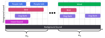Figure 1: Illustration of the concept drifts in an acoustic scene audio at a park

The change in the incoming data at  depends on a variety of different internal or external influences (e.g., event sounds that exist in a park depending on the season). The initial data recorded in the winter may only consist of people talking, bird calls, and dogs barking. However, the event sounds change in the summer, and new event sounds, such as insect and wind sounds, emerge.

2.2. Concept Drift Detection Methods

Several methods have been proposed to detect concept drifts from a data stream. This study focuses on window-based methods that use fixed windows as a reference for summarizing previous information. This approach has more accurate results than other more straightforward methods, such as cumulative sum [16]. However, the computational time and space used are higher [17]. This approach usually utilizes statistical tests or mathematical inequalities to compute the change in data. Some of the state-of-the-art methods used in this paper is presented below:

• ADWIN is a sliding window-based concept drift detection algorithm. The size of ADWIN windows might change depending on the instance in the Its size increases when the instance in the stream continues in the same distribution.  shrinks when distribution changes occur [9]. ADWIN detects concept drifts when the averages between these windows are higher than a given threshold.
• The HDDM is a concept drift detection algorithm based on fixed windows and probability inequalities [10]. The author proposes two types of HDDM, namely HDDMA and HDDMW. The HDDMA uses moving averages, whereas the HDDMW uses weighted moving averages to detect the concept drift. The HDDMA is suitable for detecting the abrupt concept drift, whereas the HDDMW is suitable for detecting the gradual concept drift.
• KSWIN [18] is a window-based concept drift detection method that utilizes the Kolmogorov–Smirnov statistic test (KS-Test) to compare the distances of two distributions. This test is a non-parametric test that does not require any assumptions about the underlying data distribution.

      Each method has its optimal hyperparameters, which differ based on the datasets used and the type of drift in those datasets.

2.3. Merging Gaussian Mixture Component

A component of a Gaussian distribution is represented by  and  to denote a mixture of  Gaussian components, where , , and  are the weight or prior probability, distribution means, and covariance matrix, respectively. This mixture must satisfy  and has the pdf defined in Eq. (2).

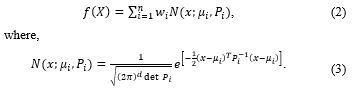
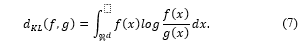
Suppose we wish to merge two Gaussian components  where , and approximate the result as a single Gaussian. The new Gaussian candidate ( ) must preserve the zeroth-, first-, and second-order moments of the original Gaussian. The moment-preserving merge is shown in Eqs. (4)–(6).

2.4. Kullback–Leibler (KL) Dissimilarity

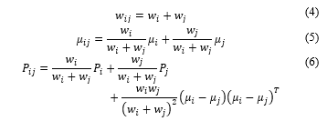
Kullback–Leibler (KL) discrimination, known as KL divergence or relative entropy, is a tool for measuring the discrepancy between two probability distributions. The KL discrimination between , a probability distribution for random variables  and , another probability distribution is the expected value of the log-likelihood ratio. The KL divergence of  and  is defined in Eq. (7), where  is the sample space of the random variable .

Based on Eq. (7), KL is not a perfect distance metric because it is asymmetric and does not satisfy the triangle inequality, . However, we can use it as metric distance because the KL discrimination of two probability distributions is larger than zero, , and the discrimination of the identical two probability distributions is zero, .

Accordingly, we apply the KL dissimilarity by computing the Kullback–Leibler discrimination upper bound of the post-merge mixture with respect to the pre-merge mixture. In the case of the Gaussian mixture, where  =  and , the KL dissimilarity between  and is shown in Eq. (8).

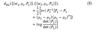Please refer to [19] for more details about the KL dissimilarity of the Gaussian distributions.

3. Proposed Method

This study extends the combine–merge Gaussian mixture model (CMGMM) [7] to classify audio scenes in concept drift situations. The CMGMM was developed based on the GMM algorithm that can incrementally adapt to the new identified component. This algorithm can add new components as new concepts and update existing components as a response to the change of the current existing concept in the current data. The CMGMM implementation is available in our public repository[1], with the algorithm pipeline shown in Figure 2.

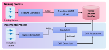Figure 2: Combine–merge Gaussian mixture model (CMGMM) general workflow

In the training process, we extract the feature of the scene audio from the training dataset  and train an optimal model . We use the Expectation maximization (EM) [20] algorithm to train the model and the Bayesian information criterion (BIC) [21] to select the best model.

In the incremental process, the performance is observed through the prediction likelihood. When KD3 detects a significant likelihood change, the model activates the concept drift adaptation process. The concept drift adaptation process then begins by creating a local model  from the new coming data.  represents the new concepts or concept updates in the incoming data. Finally, we combine the  and  components to include any new concepts from  that may not exist in the  at the initial training and merge similar components to update the existing component in .

The CMGMM pipeline process is detailed in the subsections that follow.

3.1. Feature Extraction

Feature extraction is the first step of both the training and incremental processes. In this research, we use normalized Mel-frequency cepstral coefficients (MFCCs) that represent the short-term power spectrum of audio in the frequency domain of the Mel scale. MFCCs are commonly used as features in audio processing and speech recognition. The first step is pre-emphasis for enhancing the quantity of energy in high frequencies. The next step is windowing the signal and computing the fast Fourier transformation to transform the sample from the time domain to the frequency domain. Subsequently, the frequencies are wrapped on a Mel scale, and the inverse DCT is applied [22]. Finally, each of the MFCCs is normalized using mean and variance normalization based on Eq. (9):

where,  and  denote the mean and the standard deviation of the training samples, respectively.

3.2. Model Training

The training process is intended to build a set of models from the training dataset  containing training data , where  denotes the MFCC vector. The models are trained times using the EM algorithm. For each training cycle, a different number of components  ranging from K_min to K_max is used, where  = K_max − K_min. Consequently, a set of models  is obtained based on the different numbers of components.

The next step is model selection using the BIC. In [23], the BIC value of a model  trained over the dataset X with K components, BIC(X, ), is defined as follows:

where, L denotes the model likelihood;  denotes the degree of freedom of the model parameters; and  denotes the number of training data points. The model with the lowest BIC value is selected because it maximizes the log-likelihood [6]. Algorithm 1 presents the steps of the learning process.

Algorithm 1: Training the Optimal Model
Input: Initial Dataset Dinit, Minimum Component Number Kmin, and Maximum Component Number Kmax Result: Best GMM Model
BICbest = ∞
for Kmin to Kmax do
	Mcandidate= EMTrain(Dinit, k) BICcandidate = ComputeBIC (Dinit, Mcandidate)
	if BICcandidate < BICbest then
		Mbest = Mcandidate
	End
end return Mbest

3.3. Concept Drift Detection

We propose Kernel Density Drift Detection (KD3) to detect the concept drift. KD3 is a window-based algorithm for concept drift detection. It works based on estimating the window density using the Kernel Density Estimation (KDE) or the Parzen’s window [24]. The KDE is a non-parametric probability density estimator that automatically estimates the shape of the data density without assuming the underlying distribution. The concept drift can be detected by comparing the probability functions between these windows. The greater the variation between the windows, the more evidence obtained for the concept drifts. Aside from detecting concept drifts, KD3 also collects data for adaptation (D_drift) by identifying a warning zone when data begin to show indications of concept drift.

KD3 requires three hyperparameters, namely α, β, and , which denote the margins for detecting the concept drift and accumulating the density distance and the window length, respectively. α is used to determine the threshold of the density variation in the concept drift, while β is employed to determine the threshold of the density variation in the warning zone. Therefore, α must be greater than β. KD3 accepts a set of likelihood windows as input.  is the current likelihood window that contains a sequence of log-likelihood  from the model prediction, =

First, this algorithm aims to estimate the density ( ) of the current  and previous  windows. Let  be the latest generated . Let  contain the -latest  from , , and let  contain the -latest  from , . To detect a concept drift, the distance  between  of  and  is computed using Eq. (11) within the bounds of  and . The bounds are computed based on the maximum and minimum values of the joined  of  and .

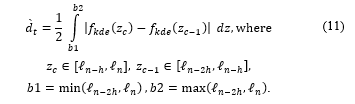Finally, the algorithm compares  to α and .hen . Suppose that the accumulative distance is equal to or greater than α. In that case, the algorithm sends the collected data to the model for adaptation. Figure 3 and Algorithm 2 illustrate the detailed KD3 process.

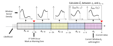Figure 3: Illustration of the Kernel density drift detection (KD3) concept

Algorithm 2: Detecting the Concept Drift
Input: Set of t likelihood , drift margin α, warning margin β (α > β), window length , Result: Drift Concept Signal, Drifted Dataset (Ddrift)
Window1 = ; Window2 = ; Bmin, Bmax = CalculateWindowBound( ); KDE1 = EstimateKDE(Window1) KDE2 = EstimateKDE(Window2) diff = distance(KDE1, KDE2, Bmin, Bmax)
if (diff ≥ α) then
	resetWarningZoneData() return true,
end if (diff ≥ β) then
	accumulativeWarning += diff
	if (accumulativeWarning ≥ α) then
		resetWarningZoneData();
		return true,
	end return false,
end return false, null

3.4. Model Adaptation

Model adaptation aims to revise the current model upon newly incoming data that might contain new concepts or concept changes. The result of this adaptation is an adapted weighted mixture component that respects the original mixture.

The model adaptation method starts by training a new model _drift from data drifts D_drift using Algorithm 1, and then combining the existing model . Consequently, the newly adapted model  accommodates the new concept represented by the components in _drift. The next step is to calculate the pairwise distance between the components in  using KL discrimination. The KL discrimination formula (Eq. (8)) enables us to set an upper bound on the discrimination of the mixture before and after the merging process. According to this formula, components with low weights means close to their variances, and similar covariance matrices are selected for merging. When two components are merged, the moment-preserving merging method [25] is used to preserve the mean and the covariance of the overall mixture (Eqs. (4)–(6)). Figure 4 illustrates the CMGM adaptation process.

Figure 4: Illustration of the combine–merge Gaussian mixture model (CMGMM) adaptation process

As a result, the reduction process generates a set of merged models _merge. To select the best _merge model, the accumulative BIC is computed by combining sampling data from _curr. D_drift then computes the BIC value using Eq. (10). The smaller the value of the accumulative BIC, the better the newly adapted model.

Based on [7] and [11], the CMGMM tends to increase the number of components because it combines and merges them. This mechanism leads to an overfitting problem because the adaptation frequency increases due to the sensitive KD3 hyperparameter.

To maintain the compactness of the CMGMM and avoid overfitting, we design a strategy to merge statistically equivalent components into one component, then prune the inactive components. The inactive components are identified by the proximity of the ratio of ² and  of the merged component to zero. In practice, components with  that are very close to zero are ignored by the model, whereas those with a large covariance tend to overlap with other components. Algorithm 3 presents in detail the steps of the proposed CMGMM-based method.

Algorithm 3: Model adaptation
Input: Current Model , Drifted Dataset Ddrift Result: Adapted Model
drift = findBestGMM(Ddrift) combine = CombineGMMComponent( drift, ) distanceMatrix = KLDissimalarity( combine) ds = Ddrift + .generateData() nCompmin = .number_component nCompmax = combine.number_component BICbest = ∞
for targetComponent = nCompmin to nCompmax
	merge = mergeComponent(target, distanceMatrix)
	if useComponentPrune then
		ComponentPrune( merge)
	End
	BICcandidate = ComputeBIC ( merge, ds)
	if BICcandidate < BICbest then
		Mbest = Mmerge
	End
end return Mbest

4. Experiment

This section provides information about the datasets and experimental setup used in this study to train, optimize, and evaluate the proposed method.

4.1. Datasets

We used three types of datasets in this experiment, that is, training, optimization, and evaluation. The training dataset consisted of audio signals extracted with a 10-seconds window from 15 scenes in the TUT Acoustic Scenes 2017 [26] and TAU Urban Acoustic Scenes 2019 datasets [26]. The scenes were home, airport, beach, office, cafe, grocery store, bus, tram, metro, city center, residential area, street pedestrian, and shopping mall.

To simulate the concept drift in the datasets, the optimization and evaluation datasets were generated by overlay new additional event sounds from and UrbanSound8K datasets [27] and the BBC Sound Class Library [28]. When the sounds were added, the numbers of additions (1–10), positions in the time axis (0–9000 ms), and loudness (−20,0) of the sounds were randomly changed at random. In total, the dataset had 46 new event classes and 371 added event sounds.

We generated four concept drift types with three scenarios. The four types of concept drift are as follows:

• abrupt concept drift (AB), where ongoing concepts are replaced with new concepts at a particular time;
• gradual concept drift (GR), where new concepts are added to an ongoing concept at a particular time;
• recurring concept drift type 1 (R1), where an ongoing concept is replaced at a particular time with concepts that previously appeared; and
• recurring concept drift type 2 (R2), where concepts that previously appeared are added to an ongoing concept at a particular time.

Figure 5 illustrates the scenario generation. The three scenarios were designed to have different data distribution complexities. The scenario details are described below:

• Scenario 1 (Sc1): A unique event sounds from a specific event sounds is repeatedly introduced with a random number of times, gain, and timing. For example, in the airport scene, unique sounds representing the airplane sound, crowd background, and construction site are overlaid with a random number of times (1–10), position (0–9000 ms), and loudness (−20,0).
• Scenario 2 (Sc2): Several event sounds are randomly selected from a set of the same sound labels in Sc1 and added using the same rule as Sc1.
• Scenario3 (Sc3): This scenario differs from Sc1 and Sc2 in that event sounds coexist among scenes. For example, a set of rain sounds exists in other scenes (e.g., beach, city center, and forest paths). The methods of selection and addition are the same as those in Sc2.

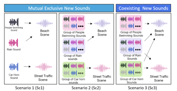Figure 5: Concept drift scenario

Table 1 shows a list of event sounds that appear at scene types in every concept drift scenario. The mutually exclusive event sounds appear in all scenarios, but coexisting sounds only appear for Sc3.

Table 1: Setting of the novel sounds in scene audio for Sc1, Sc2, and Sc3

Scene	Mutually Exclusive Sounds in Sc1, Sc2, and Sc3	Additional Coexisting Sounds in Sc3
Airport	Helicopter, crowd, and construction site	Airplane, footsteps, and children playing
Beach	People swimming, footsteps on the sand, and rain	Teenage crowd, dog, and birds
Bus	Car horn, engine, and city car	Kitchenware, phone ringing, children playing, and teenage crowd
Café /restaurant	Washing machine, food mixer, and kitchenware	Phone ringing, children playing, and teenage crowd
City center	Sound of bird, ambulance, and wind	Footsteps, phone ringing, and children playing
Grocery store	Footsteps, children playing, and shopping cart	Vacuum cleaner, phone ringing, and footstep
Home	Frying, door, and vacuum cleaner	Clock and phone ringing
Metro station	Siren, road car, and thunder	Footsteps, crowd, and wind
Office	Typing, phone ringing, and sneeze	Broom, camera, and footsteps
Public square	People running, music, and airplane	Birds, rain, and teenagers talking
Residential area	Wind, camera, and cat	Birds, sneeze, and clock
Shopping mall	Clock, camera, and teenage crowd	Children playing, phone ringing, dog
Street pedestrian	Dog, bicycle, and bird	Footsteps and children playing
Street traffic	Motorcycle, horn, and train	Siren, airplane, and bell
Tram	Coughing, bell, and footsteps on the pavement	Teenage crowd and children playing

Finally, we have one training dataset, four optimization datasets, and 12 evaluation datasets in this experiment. Each training dataset contained 3,000 scene audio, while the optimization and evaluation dataset contained 15,000 scene audio. The datasets are available in our repository[2].

4.2. Experimental Setup

The CMGMM accuracy was evaluated under four concept drift types in three scenarios (i.e., Sc1, Sc2, and Sc3). The evaluations are performed using the two following approaches:

• Active CMGMM adaptation: In this approach, the CMGMM actively detects the concept drift using a certain method and only adapts the model when the concept drift is detected. In this study, we compared KD3 to ADWIN [9], HDDMA, HDDMW [10], and KSWIN [18].
• Passive CMGMM adaptation: In this approach, the CMGMM adapts as soon as a particular datum is received without requiring the explicit prior detection of the concept drift. Several adaptation cycle sizes were tested, that is, 25, 50, 100, 150, and 200.

5. Experiment Result

The experimental result of the proposed method are presented herein.

5.1. Hyperparameter Optimization

The first step in this experiment is the systematic optimization of the KD3 hyperparameter. We used the grid-search method using a combination of hyperparameters α from 0.1 to 0.001, β from 0.0001 to 0.000001, and ɦ from 45 to 300. We prepared a particular dataset for the KD3 hyperparameter optimization in four types of concept drift.

In [11], we reported that hyperparameters β and ɦ did not have a significant effect on accuracy. Therefore, during the initial step, we observed the performance change according to β and ɦ. Figure 6 shows the average accuracy in all concept drift types according to hyperparameters β and ɦ. In this experiment, the best β and ɦ were set at 0.0001 and 45, respectively.

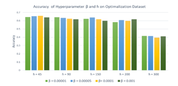Figure 6: Result of hyperparameters β and ɦ in four types of concept drift

Table 2 lists the experimental results of α in the optimization dataset in four types of concept drift. Based on this experiment, every concept drift type has its respective hyperparameter α according to the concept drift characteristics. AB and GR have similar characteristics. There are no repeating concepts in the future; hence, a more sensitive concept drift detector than R1 and R2 is required.

Table 2: KD3 hyperparameter optimization result

Concept Drift Types	Hyperparameter α (β = 0.001, ɦ = 45)
	α = 0.1	α = 0.05	α = 0.01	α = 0.005	α = 0.001
AB	0.6568	0.7113	0.7069	0.7137	0.7066
GR	0.6007	0.6173	0.7050	0.6922	0.7002
R1	0.7332	0.7232	0.7158	0.7054	0.6927
R2	0.7268	0.7133	0.7228	0.7090	0.6823
Overall	0.6793	0.6912	0.7126	0.7050	0.6950

In AB and GR, a sensitive hyperparameter α accelerated the update frequency. In the experimental result for these types of concept drifts, a high adaptation frequency reduced the loss received. However, a less-sensitive hyperparameter showed a better result in recurring concept drifts, where an old concept reappears in the future. A less-sensitive hyperparameter α provided the model with longer data compared to the sensitive hyperparameter.

We also selected the overall hyperparameter setting based on this experiment. The overall hyperparameter was selected from the best average performance of the hyperparameter optimization (α = 0.01, β = 0.001, and ɦ = 45). We used this hyperparameter for further CMGMM and KD3 evaluations.

5.2. Active Combine–Merge Gaussian Mixture Model (CMGMM) Adaptation Result

Table 3 presents the experimental results of the active CMGMM adaptation. In general, the model performance without a concept drift detector is low in all concept drift types and scenarios. The adaptations of the CMGMM on R1 and R2 showed better accuracy than those on AB and GR. On average, AB exhibited the lowest accuracy, while R2 showed the highest accuracy. This high accuracy on recurring was caused by the CMGMM being designed to preserve the old concept, even though the new concept is adapted in the model. Thus, the model can recognize the previously learned concept if it is repeated in the future.

The CMGMM experiment result depicted that KD3 outperformed other combinations in two of the four concept drift types in GR and R2. Meanwhile, ADWIN showed the best accuracy in AB. KSWIN demonstrated the best accuracy in R1, whereas HDDM was unsuitable for this case. Despite getting the highest overall accuracy score, the combination of the CMGMM and KD3 needed more frequent adaptations than ADWIN and KSWIN. In contrast, both HDDM-based methods showed worse performances compared to all others. HDDMA overdetected the concept drift in all concept drift types for more than 3000 times in GR.

The abovementioned results illustrated that the concept drift detector plays a vital role in the concept drift adaptation. The model performance decreased over time if the drift detector failed to detect or delay detecting or over detecting the concept drift.

Performance of the combine–merge Gaussian mixture model (CMGMM) and kernel density drift detection (KD3)

KD3 showed the best average accuracy of 0.6983 compared to ADWIN, KSWIN, and HDMM with 209 adaptations. This combination also showed its best results on R2 with 0.7321 accuracy, followed by R1 with 0.7373 accuracy, GR with 0.6999 accuracy, and AB with accuracy 0.6469. Furthermore, this combination was the most stable in all scenarios. The maximum performance decrements in AB, GR, R1, and R2 were 1.38%, 1.2%, 1.34%, and 0.94%, respectively.

Despite achieving a good performance in all concept drift types, the number of concept drifts detected in this combination was higher than ADWIN and KSWIN. The most significant number of adaptations occurred in AB. The disadvantage of a high number of adaptations is the higher computation time required to finish the task and possible overfitting. In this case, the higher numbers of adaptations in AB and GR are obtained because the concept constantly changes over time, and the learned concept becomes obsolete in the future; hence, the higher the adaptation, the better the performance.

Performance of the combine–merge Gaussian mixture model (CMGMM) and ADWIN

In general, the combination of CMGMM and ADWIN showed a good performance in every concept drift type, especially on the abrupt datasets, where this combination showed its best performance. The overall accuracy was 0.6371 with 83 times of adaptation. The overall accuracies of this combination in AB, GR, R1, and R2 were 0.6369, 0.6475, 0.6912, and 0.7169, respectively. Furthermore, this combination had the advantage of a small number of adaptations in all concept drift types. Hence, ADWIN showed an effective performance in using resources and had a reasonably good performance. This combination performed very well on Sc1, but showed a performance drop in Sc2 and Sc3. For example, the accuracies of AB, GR, R1, and R2 decreased in Sc3 by 4.64%, 3.82%, 2.74%, and 287%, respectively.

Performance of the combine–merge Gaussian mixture model (CMGMM) and Hoeffding’s bounds-based method (HDDM)

In this experiment, both Hoeffding’s inequality-based algorithms showed underperformance results for all concept drift types. Both algorithms were less effective in detecting the concept drift in this case. The overall accuracies of HDDMA in AB, GR, R1, and R2 were 0.4326, 0.4302, 0.494, and 0.607, respectively. The number of HDDMA adaptations exceeded 3000 times of adaptation. This high adaptation process was ineffective because the amount of trained data for each adaptation was too small. This condition led to an overfitting and decreased the model performance.

HDDM W also experienced the same problem. In some cases, HDDMA failed to detect the drift concepts, such as GR, R1, and R2 in Sc1. The overall accuracies of this HDDMW in AB, GR, R1, and R2 were 0.4347, 0.439, 0.491, and 0.5886, respectively.

Table 3: Experiment result of the CMGMM with the concept drift detector Concept Drift Detector Accuracy F1 Number of Concept Drift Detection Sc1 Sc2 Sc3 Overall Sc1 Sc2 Sc3 Overall Sc1 Sc2 Sc3 Overall AB ADWIN 0.6989 0.6525 0.6214 0.6369 0.713 0.6495 0.6353 0.6599 83 89 85 85 HDDM_A 0.4157 0.4476 0.4345 0.4326 0.4586 0.4804 0.477 0.472 3287 3350 3359 3332 HDDM_W 0.4041 0.4455 0.4546 0.4347 0.4485 0.4902 0.5004 0.4797 489 413 409 437 KD3* 0.6469 0.6359 0.6331 0.6386 0.6476 0.6467 0.6395 0.6446 207 236 220 221 KSWIN 0.6611 0.6241 0.6345 0.6317 0.6722 0.6369 0.6411 0.6501 132 121 123 125 Without Detector 0.4121 0.4054 0.4095 0.4090 0.4235 0.4125 0.4095 0.4151 GR ADWIN 0.6723 0.6341 0.6363 0.6475 0.6845 0.6506 0.6478 0.6609 92 81 83 85 HDDM_A 0.4134 0.4463 0.4311 0.4302 0.4580 0.4946 0.4701 0.4742 3306 3308 3265 3293 HDDM_W 0.4131 0.4497 0.4544 0.439 0.4524 0.487 0.4816 0.4736 0 409 401 270 KD3* 0.6999 0.6942 0.6879 0.694 0.7044 0.7004 0.6867 0.6971 190 218 221 209 KSWIN 0.6532 0.6241 0.618 0.6322 0.6631 0.6326 0.6204 0.6387 129 125 107 120 Without Detector 0.3554 0.3524 0.3489 0.3522 0.3571 0.3542 0.3501 0.3538 R1 ADWIN 0.7222 0.6948 0.6568 0.6912 0.7393 0.6981 0.6333 0.6902 78 83 87 82 HDDM_A 0.4721 0.5204 0.4896 0.494 0.5206 0.5566 0.5392 0.5388 3154 3258 3201 3204 HDDM_W 0.4847 0.4815 0.5068 0.491 0.5305 0.5215 0.5357 0.5292 0 662 647 436 KD3* 0.7373 0.7334 0.7239 0.7315 0.7389 0.7341 0.7247 0.7325 208 201 204 204 KSWIN 0.7818 0.7351 0.7357 0.7508 0.7876 0.7404 0.7416 0.7565 142 135 126 134 Without Detector 0.4512 0.4458 0.4257 0.4409 0.4512 0.4458 0.4257 0.4409 R2 ADWIN 0.7353 0.7066 0.7089 0.7169 0.7398 0.7131 0.7163 0.723 75 86 82 81 HDDM_A 0.5919 0.6034 0.6259 0.607 0.6369 0.6398 0.6658 0.6475 3052 2957 3017 3008 HDDM_W 0.5789 0.5996 0.5875 0.5886 0.6369 0.6398 0.6658 0.6475 759 604 543 635 KD3* 0.7321 0.7325 0.7227 0.7291 0.7352 0.7315 0.7221 0.7296 195 207 205 202 KSWIN 0.6914 0.6964 0.677 0.6882 0.6977 0.6976 0.6811 0.6921 156 143 141 146 Without Detector 0.4254 0.4205 0.3985 0.4148 0.4279 0.4198 0.3968 0.4148 Overall ADWIN 0.7072 0.6720 0.6559 0.6731 0.7191 0.6778 0.6581 0.6835 82 84 84 83 HDDM_A 0.4733 0.5044 0.4953 0.4910 0.5185 0.5428 0.5380 0.5331 3199 3218 3210 3209 HDDM_W 0.4702 0.4941 0.5008 0.4883 0.5170 0.5346 0.5458 0.5325 312 522 500 444 KD3* 0.7041 0.6990 0.6919 0.6983 0.7065 0.7031 0.6932 0.7009 200 215 212 209 KSWIN 0.6969 0.6699 0.6663 0.6757 0.7051 0.6768 0.6710 0.6843 139 131 124 131 Without Detector 0.4110 0.4060 0.3956 0.4042 0.4149 0.4080 0.3955 0.4061 (*) Proposed method

Performance of the combine–merge Gaussian mixture model (CMGMM) and KSWIN

The combination of CMGMM and KSWIN showed the best performance in R1, with an overall accuracy of 0.750 with 134 adaptations. The accuracies of this combination in AB, GR, R1, and R2 were 0.6317, 0.6322, 0.7508, and 0.6882, respectively. On average, KSWIN required eight to nine adaptations per scene in all dataset types. This algorithm seems able to detect occurring changes in data and supports the concept drift handling process with good indicators at a given time.

5.3. Passive Combine–Merge Gaussian Mixture Model (CMGMM) Adaptation Result

Table 4 lists the experimental results of the passive CMGMM adaptation. The best performance in AB, GR, and R1 was obtained with a cycle size of 50, and that in R2 was obtained with a cycle size of 100. The best accuracies of AB, GR, R1, and R2 were 0.7152, 0.7139, 0.7323, and 0.7155, respectively.

Table 4: The experiment result of CMGMM without concept drift detector

Concept Drift Types	Cycle Size	Accuracy
		Sc1	Sc2	Sc3	Average
AB	25	0.6290	0.6236	0.6256	0.6260
	50	0.7122	0.7159	0.7177	0.7152
	100	0.6285	0.5925	0.5955	0.6055
	150	0.6361	0.5776	0.5851	0.5996
	200	0.5580	0.5059	0.5119	0.5252
GR	25	0.6294	0.6232	0.6004	0.6176
	50	0.7133	0.7169	0.7115	0.7139
	100	0.6173	0.5887	0.6089	0.6049
	150	0.6371	0.5818	0.5797	0.5995
	200	0.5334	0.5094	0.5076	0.5168
R1	25	0.6186	0.5799	0.5608	0.5864
	50	0.7235	0.7320	0.7416	0.7323
	100	0.7211	0.7105	0.6988	0.7101
	150	0.7332	0.7086	0.7120	0.7179
	200	0.6639	0.7018	0.7146	0.6934
R2	25	0.5133	0.5444	0.5669	0.5415
	50	0.7396	0.6991	0.7011	0.7132
	100	0.7431	0.7012	0.7023	0.7155
	150	0.6865	0.6639	0.6803	0.6769
	200	0.6502	0.6011	0.6089	0.6200

Similar to active adaptation, R1 and R2 showed good performances compared to AB and GR, but better performances in passive adaptation. Although R1 exhibited the best adaptation at cycle size 50, it also showed good result at cycle sizes 100 and 150. If you consider the time and the computing resources used, then cycle sizes 100 and 150 are recommended.

In passive adaptation, the cycle size is vital in achieving a good performance. This cycle size determines the adequacy of the data for adaptation. If the cycle size is too short, the number of data adapted is small, leading to overfitting problems.

5.4. Suggestions and Limitations

The experiment results showed that the combination of CMGMM and KD3 has a higher number of adaptations compared to that of ADWIN and KSWIN due to the selection of KD3 hyperparameters that are sensitive to accommodating GR and AB. When the number of adaptations is increased, then in certain cases, such as GR and AB, the accuracy is improved, albeit with a higher computing cost. The advantage of KD3 compared to the other methods is that it could be applied in multi-dimensional probability distribution; hence, it is more flexible to apply in other models and cases.

In cases where the time or location of the concept drift can be predicted, the use of a passive adaptation strategy is more beneficial and has a lower computational cost than the active strategy. However, if the adaptation cycle is too far from the concept drift, then the model performance will decrease over time.

6. Conclusion

This paper presented KD3 hyperparameter optimization and the CMGMM performance evaluation in four types of concept drift. All concept drift types had optimum hyperparameter configurations. AB and GR showed similar patterns that required a smaller α value than the recurring concept drift. In this type of concept drift, concepts continuously appear; hence, a sensitive drift detector is needed to update the model early or have a high-frequency model adaptation. However, in recurring concepts, the new concept may be repeated in the future; thus, a lower-frequency adaptation shows a better performance.

The evaluation results demonstrated that the proposed algorithms work well in detecting and adapting to four types of concept drift and three scenarios. Overall, the CMGMM works better in R1 and R2 than in AB and GR because it is designed to preserve old concepts to preserve previously learned knowledge. Component pruning is only performed on components with a minimal impact on the prediction.

In the active adaptation strategy, the proposed combined method of CMGMM and KD3 outperformed two of four other combination methods in GR and R1. These methods showed the most stable performance among Sc1, Sc2, and Sc3 in all concept drift types. Furthermore, ADWIN showed the best results on AB. This algorithm is efficient in computing resources, but less stable in more challenging scenarios, such as Sc2 and Sc3. KSWIN showed the best results in recurring drift and good performance for all concept drift types. HDDM overdetected or failed to detect the concept drift and was not suitable in this case.

In the passive adaptation strategy, a short or long adaptation cycle could reduce the performance, and a short cycle size makes the adaptation less effective. A short cycle could disrupt the model component because the model is trained with insufficient data, leading to an underfitting problem.

In AB and GR, the model requires a high-frequency adaptation to maintain the performance; therefore, sensitive hyperparameters or a short cycle size is required. Based on the experimental results, the passive method is more suitable in these concept drift types. However, the computational costs are higher than those of the active method. Furthermore, in recurring drift scenarios, a less-sensitive hyperparameter, or a moderate cycle size is needed. The active method is recommended for recurring drift types considering the computation cost and better accuracy in experiments.

As part of our future work, we plan to improve the proposed KD3 concept drift detection algorithm to achieve adaptive weight, reduce the kernel density computation, and optimize the number of data points considered when detecting the concept drift and decreasing the computation time.

Conflict of Interest

The authors declare no conflict of interest.

Acknowledgment

This work was supported by JSPS KAKENHI Grant Number JP20K12079.

1. R. Elwell, R. Polikar, “Incremental Learning of Concept Drift in Nonstationary Environments,” IEEE Transactions on Neural Networks, 22(10), 1517–1531, 2011, doi:10.1109/TNN.2011.2160459.
2. S. Ntalampiras, “Automatic analysis of audiostreams in the concept drift environment,” in 2016 IEEE 26th International Workshop on Machine Learning for Signal Processing (MLSP), IEEE, 2016, doi:10.1109/MLSP.2016.7738905.
3. J. Gama, I. Žliobait?, A. Bifet, M. Pechenizkiy, A. Bouchachia, “A Survey on Concept Drift Adaptation,” ACM Computing Surveys, 46(4), 1–37, 2014, doi:10.1145/2523813.
4. T.R. Hoens, R. Polikar, N. V. Chawla, “Learning from Streaming Data with Concept Drift and Imbalance: An Overview,” Progress in Artificial Intelligence, 1(1), 89–101, 2012, doi:10.1007/s13748-011-0008-0.
5. I. Žliobait?, “Learning under Concept Drift: an Overview,” 1–36, 2010, doi:10.1002/sam.
6. C. Chen, C. Wang, J. Hou, M. Qi, J. Dai, Y. Zhang, P. Zhang, “Improving Accuracy of Evolving GMM under GPGPU-Friendly Block-Evolutionary Pattern,” International Journal of Pattern Recognition and Artificial Intelligence, 34(3), 1–34, 2020, doi:10.1142/S0218001420500068.
7. I.D. Id, M. Abe, S. Hara, “Concept Drift Adaptation for Acoustic Scene Classifier based on Gaussian Mixture Model,” in IEEE Region 10 Annual International Conference, Proceedings/TENCON, IEEE, Osaka: 450–455, 2020, doi:10.1109/TENCON50793.2020.9293766.
8. J.M. Acevedo-Valle, K. Trejo, C. Angulo, “Multivariate regression with incremental learning of Gaussian mixture models,” Frontiers in Artificial Intelligence and Applications, 300, 196–205, 2017, doi:10.3233/978-1-61499-806-8-196.
9. A. Bifet, R. Gavaldà, “Learning from Time-changing Data with Adaptive Windowing,” Proceedings of the 7th SIAM International Conference on Data Mining, (April), 443–448, 2007, doi:10.1137/1.9781611972771.42.
10. I. Frías-Blanco, J. Del Campo-Ávila, G. Ramos-Jiménez, R. Morales-Bueno, A. Ortiz-Díaz, Y. Caballero-Mota, “Online and Non-Parametric Drift Detection Methods Based on Hoeffding’s Bounds,” IEEE Transactions on Knowledge and Data Engineering, 27(3), 810–823, 2015, doi:10.1109/TKDE.2014.2345382.
11. I.D. Id, M. Abe, S. Hara, “Evaluation of Concept Drift Adaptation for Acoustic Scene Classifier Based on Kernel Density Drift Detection and Combine Merge Gaussian Mixture Model,” in 2021 Spring meeting of the Acoustical Society of Japan, 2021.
12. J. Montiel, J. Read, A. Bifet, T. Abdessalem, “Scikit-multiflow: A Multi-output Streaming Framework,” Journal of Machine Learning Research, 19, 1–5, 2018, doi:10.5555/3291125.3309634.
13. G.I. Webb, R. Hyde, H. Cao, H.L. Nguyen, F. Petitjean, “Characterizing Concept Drift,” Data Mining and Knowledge Discovery, 30(4), 964–994, 2016, doi:10.1007/s10618-015-0448-4.
14. T. Zhang, J. Liang, B. Ding, “Acoustic scene classification using deep CNN with fine-resolution feature,” Expert Systems with Applications, 143(1), 113067, 2020, doi:10.1016/j.eswa.2019.113067.
15. A. Tsymbal, “The Problem of Concept Drift: Definitions and Related Work,” 2004.
16. E.S. Page, “Continuous Inspection Schemes,” Biometrika, 41(1/2), 100, 1954, doi:10.2307/2333009.
17. Y. Yuan, Z. Wang, W. Wang, “Unsupervised concept drift detection based on multi-scale slide windows,” Ad Hoc Networks, 111, 102325, 2021, doi:10.1016/j.adhoc.2020.102325.
18. C. Raab, M. Heusinger, F.M. Schleif, “Reactive Soft Prototype Computing for Concept Drift Streams,” Neurocomputing, 2020, doi:10.1016/j.neucom.2019.11.111.
19. A.R. Runnalls, “Kullback-Leibler Approach to Gaussian Mixture Reduction,” IEEE Transactions on Aerospace and Electronic Systems, 43(3), 989–999, 2007, doi:10.1109/TAES.2007.4383588.
20. A.P. Dempster, N.M. Laird, D.B. Rubin, “Maximum Likelihood from Incomplete Data via the EM Algorithm,” Journal of the Royal Statistical Society. Series B (Methodological), 39(1), 1–38, 1977.
21. A.D.R. McQuarrie, C.-L. Tsai, Regression and Time Series Model Selection, WORLD SCIENTIFIC, 1998, doi:10.1142/3573.
22. P. Pal Singh, “An Approach to Extract Feature using MFCC,” IOSR Journal of Engineering, 4(8), 21–25, 2014, doi:10.9790/3021-04812125.
23. C. Fraley, “How Many Clusters? Which Clustering Method? Answers Via Model-Based Cluster Analysis,” The Computer Journal, 41(8), 578–588, 1998, doi:10.1093/comjnl/41.8.578.
24. E. Parzen, “On Estimation of a Probability Density Function and Mode,” The Annals of Mathematical Statistics, 33(3), 1065–1076, 1962, doi:10.1214/aoms/1177704472.
25. J.L. Williams, P.S. Maybeck, “Cost-function-based Gaussian mixture reduction for target tracking,” Proceedings of the 6th International Conference on Information Fusion, 2, 1047–1054, 2003, doi:10.1109/ICIF.2003.177354.
26. A. Mesaros, T. Heittola, T. Virtanen, TUT Acoustic scenes 2017, Development dataset, 2017, doi:10.5281/ZENODO.400515.
27. J. Salamon, C. Jacoby, J.P. Bello, “A Dataset and Taxonomy for Urban Sound Research,” MM 2014 – Proceedings of the 2014 ACM Conference on Multimedia, (November), 1041–1044, 2014, doi:10.1145/2647868.2655045.
28. BBC, BBC Sound Effects, https://sound-effects.bbcrewind.co.uk/search, Mar. 2019.

(Click Here)