1. Introduction

The increasing availability of large amounts of agricultural commodity prices historical data and the need of performing accurate predicting of price fluctuations in agricultural economy demands the definition of robust and efficient techniques, which are able to infer from current observations. The traditional way to solve the prediction problem lies in linear statistical methods (such as ARIMA models), and more recently with the emergence of machine learning techniques, the solution has largely shifted from statistical methods to machine learning area. However, the selection of proper machine learning techniques for automated agriculture commodity price prediction still has limited consideration. On the other hand, when implementing machine learning techniques, finding optimal parameters of learning algorithm for global solution, nonlinearity and avoiding curse of dimensionality are still biggest challenges, therefore machine learning strategies studies are needed.

In practice, volatility in price of agricultural commodities is often unpredictable as they are affected by eventualities for example fluctuations of oil price, greenhouse effects and natural disasters such as flood or attacks by disease. Uncertainties of agricultural commodities price endanger the accessibility of food by consumers which leads to food insecurity and causes starvation and malnutrition. Instability of agricultural commodities price due to oversupply or lack of demand causes unnecessary food wastage. In recent years, the price of some agricultural commodities (such as palm oil and rubber) has been steadily decreased. This downward trend is making an impact to Malaysia’s economy and can contribute to a slower economic growth in various investments in Malaysia. There are many exogenous factors that could cause such a trend and time-series data analysis is required to forecast this trend to improve Malaysia’s agricultural plantation plan for better country development. Being able to anticipate the fluctuations and patterns in agricultural commodities price will enable the government to propose new policies that can help prevent the country into worse economy state. Further, the agricultural commodities providers are able to control their supply based on the time series analysis in order to prevent a bad plantation plan.

Most of the time series analysis on agricultural commodities are based on the US and China commodities market and there is no concrete research done about the Malaysia commodities market. Therefore, thorough agricultural commodities prices analysis should be performed based on the Malaysia prices.

In this research, we address these problems by conducting a machine learning strategy study and propose a web-based automated system to predict agriculture commodity price.

The main contribution of our work is summarized as follows:

• We formulate prediction of agriculture commodity price as a machine learning problem, which is more accurate, robust and efficient with the increasing availability of large amounts of agricultural commodity prices historical data than the traditional statistical methods.
• The proposed web-based automated agriculture commodity price prediction system with the best performance machine learning model has been presented as an advanced solution to fulfill the need of performing accurate predicting of price fluctuations in agricultural economy demands.
• Five popular machine learning algorithms, ARIMA, SVR, Prophet, XGBoost and LSTM have been compared with large historical datasets in Malaysia, which could serve as the foundation for other Malaysia commodities market research.

This paper is an extension of work originally presented in ITCC 2020 [1].

2. Background

In the earliest studies, the focus of analysis is on commodity futures markets. William G et al. discovered that futures prices were good price predictors in the corn, soybean and potato market established from empirical forecast assessment [2]. Many other subsequent studies on different agricultural futures markets in 1970’s was the result of high dependency used by the researchers, who were interested in specific market conditions and traditional econometric models [3]. However, there are two obvious problems when implementing the traditional econometric models in the earliest days. First is the limited analysis due to the capacity of the model and  the high computational cost [4], [5]. Second is those models are estimated through assumption that variables are independent, normal distribution, which is unrealistic in the real world [6].

Later on, several research studies have been proposed to implement agriculture price prediction scheme using different machine learning algorithms [7]-[10]. However, the performance of machine learning in agricultural commodity futures prediction is rarely explored. Future forecasting is usually done by analysing past price data of each commodity, climate, location, planting area, and several other conditions. Therefore, it is challenging because of its inherent complexity and dynamism. According to the lowest error percentage, many researchers have selected ANN and PLS as prediction algorithms.

Table 1: Summary of Related Work

Article	Agriculture Commodities	Technique
Tomek et al. [2]	Corn, Soybean, Potato	Empirical Forecast Assessment: Linear Regression
Kofi et al. [3]	Wheat, Potato	Traditional Econometric Model: Linear Regression
Sariannidis et al. [4]	Rice	Statistical Models: Autoregressive Conditional Heteroskedasticity (ARC), Generalized Autoregressive Conditional Heteroskedasticity (GARC)
Zulauf et al. [5]	Corn, Soybean	Econometric models: Price-level and Percent-change Models
Onour et al. [6]	Wheat, Rice, Beef, Groundnut, Sugar, coffee	Statistical Models: ARC/GARC models, Stochastic Volatility (SV) models.
Xiong et al. [7]	Cotton, Corn	Vector Error Correction model (VECM) – multi-output support vector regression (MSVR)
Peng et al. [8]	Cabbage, Bok choy, Watermelon, Cauliflower	Autoregressive Integrated Moving Average (ARIMA),  Partial Least Square (PLS), and Artificial Neural Network (ANN)
Kumar et al. [9]	Sugarcane	K-Nearest Neighbor, Support Vector Machine (SVM),  Least Squared Support Vector Machine
Manjula et al. [10]	—	Optimal Neural Network classifier (ONN)
Cao et al. [11]	—	SVM, RBF neural network
Connor et al. [12]	—	Recurrent Neural Networks
Dasgupta et al. [13]	—	Gaussian Dynamic Boltzmann Machine (DyBM) model with a recurrent neural network (RNN)
Tang et al. [14]	—	Feed Forward, Backpropagation Neural Network models, Standard Box-Jenkins model
Namaki et al. [15]	—	Deep Neural Network
Siami-Namini et al. [16]	—	Long Short-Term Memory (LSTM), Autoregressive Integrated Moving Average (ARIMA)
Hochreiter et al. [17]	—	Long Short-Term Memory (LSTM)
Chen [1]	Chicken, Chili, Tomato	ARIMA, SVR, Prophet, XGBoost and LSTM

In [9], the author proposed a system to apply prediction by analyzing past soil and rainfall datasets. In another research paper, Askunuri Manjula [10] has done crop prediction using multiple features, such as weather forecasting, pesticides and fertilizers and past revenue. Both of these two research works have been done the prediction with implementing pre-processing and feature reduction functions.

A few research studies have focused on implementing neural networks for prediction [11]-[13]. However most of these works are mainly about interval prediction and the point forecasting of agricultural commodity prediction has been taken less notice. Further on, because of gradient vanishing, these existing methods fail to capture very long-term information [11]. Next, the dynamic dependencies among multiple variables are not being taken into consideration [12]. Besides that, these studies fall short in distinguishing a mixture of short-term and long-term repeating patterns explicitly [13].

During the recent years, research works of the promising deep neural networks algorithms in time series forecasting can be classified into three categories [14]. First category is to identify statistically significant events; the second is to find and predict inherent structure and the third is to do accurate prediction on numerical value [15]. Looking into time series prediction through deep neural networks, the most popular approach is Long Short Term Memory (LSTM). This approach has been highly discussed due to its promising result and the capability of not only modelling nonlinear patterns, realizing complex causal relationships, as well as the learning rate on huge historical datasets. The LSTM model is said to be more accurate than the prediction of the ARIMA model by 85% on average from the results obtained in the research by Namini, S. S, Tavakoli, N. and Namin, A. S [16]. Furthermore, LSTM were introduced and aimed for a better performance by tackling the vanishing gradient issue that recurrent networks would suffer when dealing with long data sequences [17].

Other advance technologies, such as Box–Jenkins approach [18] and irrigation monitoring systems based on IoT technologies, GPS and LoRaWAN [19] have been presented by researchers recently. However due to the application in different domain or system complexity, we will not consider these techniques in this paper but it might be useful for our future work.

A summary of all these related works can be found in Table 1. Other background information and technical review of ARIMA, SVR, Prophet, XGBoost and LSTM have been discussed in our conference paper [1].

3. Proposed System

The main objective of the proposed automated agriculture commodity price prediction system is to assist government or farmers for a better agricultural plantation plan. To achieve the objective, this research utilizes machine learning techniques to provide an agriculture price forecasting feature into the web system.

The project studies the needs of the farmers in doing agricultural activities, and these studies have been adapted into the system and be delivered in a simpler, more comprehensive way to suffice the farmers’ knowledge in doing agricultural activities.

3.1. System Requirement Specification

3.1.1. Functional Requirements

The system should have a web app which consists of:

• A sign up and login page
• A forecast page to show all graph and data
• A commodity information page
• A user profile page
• An enquiry page

The system should forecast the future prices of agriculture commodities

• The forecast should be shown in a graph form
• User should be able to choose duration of prediction
• User should be able to rescale the x-axis of the graph
• The forecast should be based on previously available data
• User shall be able to access different type of model in price forecast (Univariate / multivariate)
• Graph should be updated upon type of commodity, duration of view, forecast period, and type of model

Visualization of forecast result should be clear for users

• Past prices and forecast results shall be separated with different color in one graph
• When the cursor hovers above the graph line, price information of the x-axis value shall be shown to users

Users shall able to select interested commodity

• Commodity chosen can only be pre-existing in the database
• System should update graph to show new data point based on new data added
• User shall be able to access different model type for each commodity (univariate, multivariate)

System should store and retrieve data in a database

• Developers should be able to update the database with new data
• Developers should be able to edit previous data stored in the database

Commodities data shall be downloadable

• User shall be able to download complete past prices of selected commodities in .csv file

A user profile shall be created automatically upon registration

• User shall be able to edit the user profile and save it

System shall be able to authenticate existing user

• User account shall be saved in database during registration

3.1.2. Non-Functional Requirements

Reliability

• The system shall be able to access the system anywhere with an internet connection
• The system shall be able to handle user queries not exceed 30 seconds when Tensorflow backend is running

Usability

• The system shall be simple to access for a first-time user
• The redirecting page amount for any feature of the system shall not exceed 5 pages

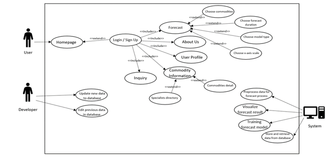Figure 1: Use Case Diagram of the Automated Agriculture Commodity Price Prediction System

Performance

• The forecasting result shall be available for at least 7 commodities
• For each commodity, univariate model and multivariate model for forecast process shall be able to be accessed
• The meantime of download a file in csv format from a software shall not exceed 10 seconds

Security

• The system would require user account to access to all features
• User shall register their account with their email address one time only, system will reject account registration of existing account

  Commodity products

• Commodities listed in the software shall be in English
• All commodities prices in the software shall be in Ringgit Malaysia, and local pricing for every commodities

Interface

• The system shall be portable in devices including personal computers, iPad and any mobile devices with Google Chrome software installed.
• The system layout shall be responsive to both full-size window and minimized window

3.2. Use Case Diagram

The use case diagram is shown in Figure 1. It explains the interactions that occur between the users and the system itself.

3.3. System Overview

Figure 2 describes the system Flow. The web system follows the Model-View-Controller (MVC) architecture. When a user enters a URL in their browser, the browser sends an http request to the web server, then the web server forwards the request to the application server and the URL setting contained in the urls.py file selects the view according to the url specified in the request, the view communicates with the database via models.py, renders the html or other format using templates (loads the static files) and returns the http response to the web server and finally, the web server provides the desired page to the browser.

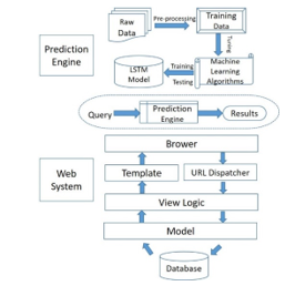Figure 2: System Flow of the Automated Agriculture Commodity Price Prediction System

3.4. Prediction Engine Design

There are four processes in the prediction engine design of the proposed system: data pre-processing process, tuning process, training and testing process and decision-making process. Process 1 involves cleaning and reformatting the dataset; while process 2 focuses on defining optimal parameter value of each machine learning techniques. All machine learning models will be trained and tested in process 3. Five machine learning methods were compared in this research, which are ARIMA [20], SVR [21], Prophet [22], XGBoost [23] and LSTM [17]. Technical details of these methods have been presented in our conference paper [1]. Finally, process 4 selects the best model out of all models to serve as the prediction engine. An algorithm snippet of the prediction engine is shown in Figure 3.

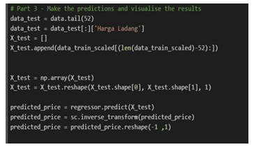Figure 3: Algorithm snippet of the prediction engine

3.5. Implementation Practice

The main implementation of the application for machine learning algorithms to predict is Python programming language. It is an interpreted, high-level, general-purpose programming language used widely for machine learning. For the frontend design implementation of the application, Hypertext Markup Language (HTML), Cascading Style Sheets (CSS) and JavaScript have been used. These are high-level languages widely used to build a design and features of web applications.

3.5.1. Collaborative Software and Version Control

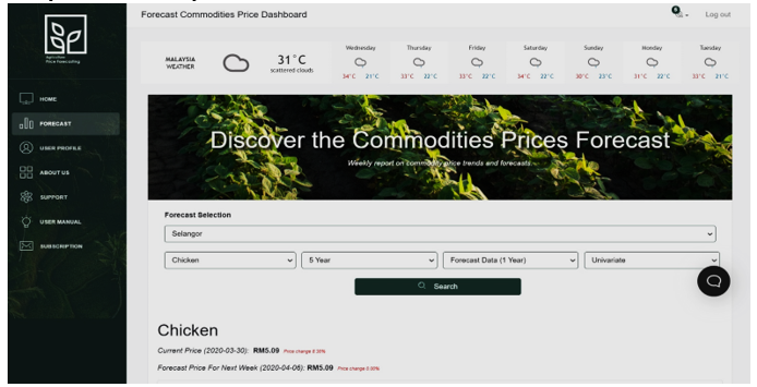Figure 4: Forecasting Page of the Automated Agriculture Commodity Price Prediction System

Django is the main framework used to build our web application, which is Python-based software that follows the model-template-view architectural pattern. Besides, a free cloud service which supports free GPU named Google Colab is in service to assist while implementing Long short-term memory (LSTM) algorithms in python programming language and it also supports the development for deep learning applications using popular libraries such as TensorFlow, Keras, PyTorch and  so on.

Github, an open source version control website, is used as a centralized repository to keep, share, update codes and most importantly is to do version control. This platform is used as our service-oriented architecture for the application, also to manage the codebased, deliver the latest code and manage configuration of our web application.

3.5.2. Graphical User Interface (GUI)

During the initial implementation to achieve our prototype user interface (UI), we have used Hypertext Markup Language (HTML) to build the main structure of the homepage, login page and the forecasting dashboard. Thus, we modify using Cascading Style Sheet (CSS) and JavaScript to implement our proposed design accordingly.

In the latest design, there are 8 pages that build up the website, particularly, register, login, dashboard, user profile, support, weather forecast, about us and subscription page. Firstly, the user will be required to have an account in order to login the page, this will be handled in the register page for the user to create an account. Secondly, after getting an account, the user will be redirected to the login page with a simple input form for the user to log in with their account. All of the pages will require the user to login in order to view it. After logging in, there will be a side navigation bar containing each Uniform Resource Locator (URL) for relevant pages. In the forecast page as shown in Figure 4, users will be allowed to view the forecast result as a graph and users will also be able to select relevant commodities, data types, and duration of forecast they would prefer to see in the graph. The user profile will handle all the information that belongs to the user and users will be able to edit and update their profiles. In the support page, users may submit their enquiries via the form provided. The about us page is a brief introduction regarding the website and its purpose and usage. In the subscription page, the user will be able to subscribe to different plans to unlock different features. Lastly, each page contains the identical top navigation bar for them to log out anytime.

4. Experiments and Results

The forecasting feature of the prediction system is the main focus of the project. In the decision of technique implemented to serve as the prediction engine, a series of experiments have been designed to discover the most optimal algorithm which should perform with highest accuracy and best capability of handling increasing data.

Based on our literature review analysis, five algorithms namely, ARIMA, SVR, Prophet, XGBoost and Long short-term memory have been selected as our potential prediction engine and their performance will be compared to learn the best model of interest from large datasets.

4.1. Datasets

Our experimental agriculture datasets are extracted from the report made by FAMA official government website (https://sdvi.fama.gov.my/analisahargamingguan/DownloadPass word.asp). This website consists of weekly data analysis reports from 2007-2020. The price datasets of different categories (December 2008 to March 2020) are selected and migrated into a raw dataset. Two series of experiments have been conducted, one is to consider only time-series dataset with 11 years’ datasets (December 2008 to March 2019) and the other is with multivariable (Temperature, Humidity, Precipitation and Crude Oil Price) with the whole dataset.

Table 2 shows the statistics of the price with three selected   commodities from two categories, chicken for poultry, chili and tomato for fruits. All three commodities datasets with 2% missing values.

Table 2: Price Statistics of the Raw Data

Commodities	Mean	Minimum	Maximum	StdDev
Chicken	4.84	3.50	6.25	0.52
Chili	5.92	2.90	12	1.55
Tomato	2.19	0.50	6.35	0.83

4.2. Experimental Setting

4.2.1. Configuration of ARIMA

ARIMA is a combination of two models that is Auto regressive (AR) and moving average (MA). ARIMA consists of three parameters (p,d,q), where: p is the number of autoregressive terms, d is the number of nonseasonal differences needed for stationarity, and q is the number of lagged forecast errors in the prediction equation [20]. A series of actions have been performed to preprocess the data. Firstly, an Augmented Dickey Fuller Test (ADCF) is performed to determine whether the time series is stationary and perform data transformation to assure the stationarity of the data [22]. And then a differencing method is used to transform a non-stationary time series into a stationary one, a lag of 1 has been given as the result shows that the mean and variance are more constant over time in comparison to before transformation, thus resulting in ARIMA (d,1).

 AR demonstrates the correlation between the previous time period with the current. Thus, in order to predict the value of P, a partial auto-correlation function (PACF) graph will plot. This plot provides a summary of the relationship between an observation in a time series with observations at prior time steps with the relationships of intervening observations removed [25].

Inevitably, there is always noise or irregularity attached in a time series. Hence, MA has been implemented and the main purpose is to figure and average out the noises that could potentially affect the model. This has been achieved by plotting an Auto Correlation Function (ACF) autocorrelation plot. An ACF plot is an (complete) auto-correlation function which gives values of auto-correlation of any series with its lagged values, it describes how well the present value of the series is related with its past values [24][26]. From our experimental results, it is observed that the diagram shows that the graph cuts off and drops to zero for the first time on x-axis in 1 on ACF plot and 1.5 on ACF plot, thus, giving q=1 and p=1.5.

4.2.2. Configuration of SVR

To capture the non-linear pattern of the data prediction, the implemented SVR model has used Radial Basis Function as the kernel function. As a popular function used in most kernelling algorithm, it was claimed of having well performance under general smoothness assumptions [27] and this suits the situation in our study. All parameter settings remain default, however, some parameter values have been tuned in building the model, such as:

• The kernel coefficient (gamma) setting value is set as 1/total number of features to deal with various amounts of features.
• Regulation parameter(C) is set by fine-tuning to find the most suitable value for the model.
• The epsilon setting is used with default value.

To resolve the missing values, two different approaches have been implemented to the model:

• The missing value in the initial raw data – fill the missing value with valid, but not influence value (e.g. -99999) to avoid clearance of missing data affecting the prediction process.
• The missing value in the post-process raw data – clear the missing data to maintain the same amount of row in the data frame.

Training of the model has utilized the python sklearn function called train_test_split. The dataset is randomly split into the corresponding train set and test set, in this case, the ratio of training set and test set is 9:1.

4.2.3. Configuration of Prophet

The default setting of Prophet:

• growth (‘linear’)
• changepoints (n)
• range (0.8)
• changepoint_prior_scale (m)

The number of change points n has been set as one per month. The changepoint_prior_scale is to decide how flexible the changepoints are allowed. To avoid the overfitting problem, m has to set to [10,30]. Prophet is relatively robust to missing data, so no resampling methods have been implemented. Cross-validation method has been implemented to split the date into training and testing sets.

4.2.4. Configuration of XGBoost

The default setting of XGBoost:

• objective=’reg:linear’,
• colsample_bytree=0.8,
• learning_rate=0.1,
• max_depth=8,
• n_estimators=1000,
• silent=1,
• subsample=0.8,
• scale_pos_weight=1,
• seed=27
• early_stopping_rounds=50

4.2.5. Configuration of LSTM

The default setting of LSTM:

• Number of epochs: 100
• Batch size: 10
• Layers: 4 LSTM layer (including input layer) each of size 50 unit and subsequent by a dropout layer of +/-2 based on the dataset after each layer. 1 Output dense layer of size 52.
• Optimizer and loss function: adam, mse.
• Activation: hyperbolic tangent
• Data transform: data are scaled by a minmaxscaler

4.3. Results

The final mean squared error score (MSE) for the prediction in the first series of experiments has been shown in Figure 5. The mean squared error score gives a better justification of the optimal algorithm that could be chosen as the prediction engine. From the results, ARIMA has shown as the most stable model amongst the three commodities, as it has the lowest mean square error value (0.251) on average, particularly with Chili, it gets as low as 0.027 for MSE.

From the literature review, LSTM is more superior than other machine learning models such as SVR and ARIMA in terms of accuracy and difficulties in handling the data. However, in the first series of experiments, due to the small sample size, it was not able to perform outstanding predictions to fit the system. We can conclude ARIMA has outstanding ability in handling small amounts of data in performing predictions.

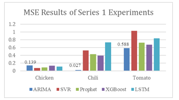Figure 5: MSE Results of Series 1 Experiments

In order to test the longer term of agriculture commodity price prediction, which is more approximate to the real world situation,   a second series of experiments have been conducted. In the second attempt of the experiment, the data has been enlarged to March 2020, and the feature space has been increased from one dimension to multi-dimensions with Temperature, Humidity, Precipitation and Crude Oil Price features being added to the model training process. Figure 6 shows the latest results of the second series of experiments.

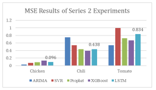Figure 6: MSE Results of Series 2 Experiments

From the results, the average performance of LSTM with MSE has improved 45.5% while ARIMA has dropped 74.1%. The average MSE of LSTM is 0.304 which outperformed all other four algorithms. The improvement of the LSTM model shows its potential in handling increasing data and higher complexity of data compared to other models and in a long-term overview. Considering the fact that the collected data will continuously increase in terms of size and complexity, hence, LSTM is a better choice comparing to ARIMA (which shows the best result in the first series of experiment). Meanwhile LSTM’s outperform capability of handling bigger dataset, as well as in the terms of system maintainability and scalability have fully justified the suitability to serve as the prediction engine for the proposed automated agriculture commodity price prediction system.

Figure 7 (a) to (c) are the graphs that illustrate the original prices, as well as the prediction prices using LSTM algorithm for 3 experimental commodities (Chicken, Chilli and tomato). The graph can help to visualise the outcome of predicted price in order to make a visual presentation to users.

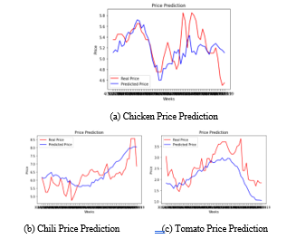Figure 7: LSTM Prediction Results

5. Conclusion

In this research, we study the challenges of prediction on price fluctuations in agricultural economy with increasing large amounts of agricultural commodity prices historical data.  An accurate, robust and efficient agriculture commodity price prediction system with novel machine learning techniques have been proposed, which is able to automatically infer from current observations. The traditional way to solve the prediction problem lies in linear statistical methods (such as ARIMA models), and in this paper we present the novel and complete solution in machine learning area.

Firstly, the prediction of agriculture commodity price has been formulated as a machine learning problem. It is more accurate, robust and efficient for the increasing availability of large amounts of agricultural commodity prices historical data than the traditional statistical methods. Secondly the proposed web-based automated agriculture commodity price prediction system with the best performance machine learning model engine has been presented as an advanced solution for the need of performing accurate predicting of price fluctuations in agricultural economy demands. Thirdly five popular machine learning algorithms, ARIMA, SVR, Prophet, XGBoost and LSTM have been compared with large historical agriculture commodity price datasets in Malaysia, which could serve as the foundation for other Malaysia commodities market research.

In future, correlation analysis between different supporting factors and the historical price will be investigated in depth and the optimization of the proposed prediction engine model will be further improved. The proposed system will also enhance its trading aspect in near future, by reporting more in-depth location-specific price analysis to realize trading among farmers.

Conflict of Interest

The authors declare no conflict of interest.

Acknowledgment

This paper is part of a research funded by the Ministry of Higher Education Malaysia under the Fundamental Research Grant Scheme (FRGS/1/2018/ICT02/UNIM/02/1).

1. Z.Y. Chen, K.L.Sin, “Long Short-Term Memory Model Based Agriculture Commodity Price Prediction Application,” in Proceedings of the 2020 2nd International Conference on Information Technology and Computer Communications, Association for Computing Machinery, New York, NY, USA: 43–49, 2020, doi: https://doi.org/10.1145/3417473.3417481.
2. W.G. Tomek, R.W. Gray, “Temporal Relationships Among Prices on Commodity Futures Markets: Their Allocative and Stabilizing Roles,” American Journal of Agricultural Economics, 52(3), 372–380, 1970, doi:https://doi.org/10.2307/1237388.
3. T.A. Kofi, “A Framework for Comparing the Efficiency of Futures Markets,” American Journal of Agricultural Economics, 55(4_Part_1), 584–594, 1973, doi:https://doi.org/10.2307/1238343.
4. N. Sariannidis, E. Zafeiriou, “The spillover effect of financial factors on the inferior rice market,” Journal of Food, Agriculture & Environment, 9(1), 336–341, 2011, doi:https://doi.org/10.1234/4.2011.1962.
5. C.R. Zulauf, S.H. Irwin, J.E. Ropp, A.J. Sberna, “A reappraisal of the forecasting performance of corn and soybean new crop futures,” Journal of Futures Markets, 19(5), 603618, 1999, doi:https://doi.org/10.1002/(SICI)1096-9934(199908)19:5<603::AID-FUT6>3.0.CO;2-U.
6. I. Onour, B.S. Sergi, “Modeling and Forecasting Volatility in the Global Food Commodity Prices (Modelování a Prognózování Volatility Globálních cen Potraviná?sky?ch Komodit),” Agricultural Economics-Czech, 57(3), 132–139, 2011, doi:https://doi.org/10.17221/28/2010-AGRICECON.
7. T. Xiong, C. Li, Y. Bao, Z. Hu, L. Zhang, “A combination method for interval forecasting of agricultural commodity futures prices,” Knowledge-Based Systems,77,92–102, 2015, doi:https://doi.org/10.1016/j.knosys.2015.01.002.
8. Y.-H. Peng, C.-S. Hsu, P.-C. Huang, “Developing crop price forecasting service using open data from Taiwan markets,” in 2015 Conference on Technologies and Applications of Artificial Intelligence (TAAI), 172–175, 2015, doi: https://doi.org/10.1109/TAAI.2015.7407108.
9. A. Kumar, N. Kumar, V. Vats, “Efficient crop yield prediction using machine learning algorithms,” International Research Journal of Engineering and Technology,5(06),3151–3159,2018. Online Access.
10. A. Manjula, G. Narsimha, “Crop Yield prediction with aid of optimal neural network in spatial data mining: New approaches,” International Journal of Information and Computation Technology, 1(6), 25–33, 2016. Online Access.
11. L.J. Cao, F.E.H. Tay, “Support vector machine with adaptive parameters in financial time series forecasting,” IEEE Transactions on Neural Networks, 14(6), 1506–1518, 2003, doi:https://doi.org/10.1109/TNN.2003.820556.
12. J. Connor, L.E. Atlas, D.R. Martin, “Recurrent networks and NARMA modeling,” in Advances in neural information processing systems, 301–308, 1992, doi:https://dl.acm.org/doi/10.5555/2986916.2986953.
13. S. Dasgupta, T. Osogami, “Nonlinear Dynamic Boltzmann Machines for Time-Series Prediction,” Proceedings of the AAAI Conference on Artificial Intelligence,31(1),2017,doi:https://dl.acm.org/doi/10.5555/3298483.3298506.
14. Z. Tang, C. de Almeida, P.A. Fishwick, “Time series forecasting using neural networks vs. Box- Jenkins methodology,” SIMULATION, 57(5), 303–310, 1991, doi:https://doi.org/10.1177/003754979105700508.
15. M.H. Namaki, P. Lin, Y. Wu, “Event pattern discovery by keywords in graph streams,” in 2017 IEEE International Conference on Big Data (Big Data), 982–987, 2017, doi: https://doi.org/10.1109/BigData.2017.8258019.
16. S. Siami-Namini, N. Tavakoli, A. Siami Namin, “A Comparison of ARIMA and LSTM in Forecasting Time Series,” in 2018 17th IEEE International Conference on Machine Learning and Applications (ICMLA), 1394–1401, 2018, doi: https://doi.org/10.1109/ICMLA.2018.00227.
17. S. Hochreiter, J. Schmidhuber, “Long Short-Term Memory,” Neural Computation,9(8),1735-1780,1997, doi:https://doi.org/10.1162/neco.1997.9.8.1735.
18. A.M. Ashik, K.S.Kannan, “Time Series Model for Stock Price Forecasting in India”, in Logistics, Supply Chain and Financial Predictive Analytics. Asset Analytics (Performance and Safety Management). Springer, Singapore, 2018, https://doi.org/10.1007/978-981-13-0872-7_17.
19. D. M. Matilla, Á. L. Murciego, D. M. Jiménez Bravo, A. Sales Mendes and V. R. Quietinho Leithardt, “Low cost center pivot irrigation monitoring systems based on IoT and LoRaWAN technologies,” 2020 IEEE International Workshop on Metrology for Agriculture and Forestry (MetroAgriFor), 2020, 262-267, doi: 10.1109/MetroAgriFor50201.2020.9277548.
20. G.E.P. Box, G. Jenkins, Time Series Analysis, Forecasting and Control, Holden-Day, Inc., USA, 1990, doi:https://dl.acm.org/doi/10.5555/574978.
21. M. Awad, R. Khanna, Support vector regression, Springer: 67–80, 2015, doi:https://doi.org/10.1007/978-1-4302-5990-9_4.
22. S.J. Taylor, B. Letham, “Forecasting at Scale,” The American Statistician, 72(1), 37–45, 2018, doi:https://doi.org/10.1080/00031305.2017.1380080.
23. T. Chen, C. Guestrin, “XGBoost: A Scalable Tree Boosting System,” in Proceedings of the 22nd ACM SIGKDD International Conference on Knowledge Discovery and Data Mining, Association for Computing Machinery, New York, NY, USA: 785–794, 2016, doi: https://doi.org/10.1145/2939672.2939785.
24. Y. W. Cheung, K. S. Lai, “Lag order and critical values of the augmented Dickey–Fuller test”, Journal of Business & Economic Statistics, 13(3), 277-280, 1995,doi: https://doi.org/10.1080/07350015.1995.10524601.
25. R. H. Shumway, D. S. Stoffer, Time series analysis and its applications: With R , Principles of fuel cells, Springer, 2006.
26. G. E. P. Box, W. G. Hunter, J. S. Hunter, Statistics for experimenters: an introduction to design, data analysis, and model building, John Wiley and Sons, 1978.
27. A. J. Smola, B. Schölkopf, K. R. Müller, “The connection between regularization operators and support vector kernels”, Neural networks, 11(4), 637-649, 1998, doi: 10.1016/S0893-6080(98)00032-X.

(Click Here)