1. Introduction

The global food demand in the first half of this century is expected to grow 70 percent, and if we don’t do anything there would be a major problem with food security by 2050 [1]. One of the reasons why there has been a massive demand for food is the growing population. Increased population means increased demands on food produce. Right now, there is a 7.8 billion population, and the number continues to rise. High food price was one of the reasons listed why there is a high amount of malnutrition in the world.

The three common sources of carbohydrate are rice, wheat, and corn. Countries in Asia and most of Africa and South America, eat rice as the main staple food. Based on the data by BPS in Indonesia, it shows that in 2018 the average per capita consumption of rice per week was 1.551 kg [2]. Forecasting commodity prices play an important role in the livestock or agriculture industry because it is useful for maximizing profits and minimizing risks [3], Accurate food price prediction can lead to optimization of resource allocation, increased efficiency, and increased income for the food industry [4]. The increase in food prices can become a burden, especially for the middle to the lower-income community.

Several studies have been done using the regression model, whether it being the classic linear regression or ridge regression. A study by [5] in stock market prediction uses linear regression to forecast the daily behavior of the stock market. The results show a high confidence value in linear regression compared to the other regression methods. In another  study on the prediction of wheat prices in China [6], prices are predicted using a combination of linear models. Though there are downsides that could be found in a linear model, one of them being a multicollinearity problem.

In a linear regression model, multicollinearity happens when independent factors in a relapse model are associated. This relationship is an issue since independent factors should be free. If the level of connection between factors is sufficiently high, it can cause issues when you fit the model and decipher the outcomes. Multicollinearity diminishes the accuracy of the estimated coefficients, which debilitates the statistical power of the regression model. Multicollinearity also enables the coefficient estimates to swing fiercely dependent on which other independent factors are in the model. The coefficients become delicate to little changes in the model.

To deal with multicollinearity, in [7] the author proposed a Bayesian ridge regression method and treating the bias constant. They use a conjugate and non-conjugate model while diagnosing and treating the collinearity simultaneously. They mention that the practice of dropping variables from the data is not a good practice to correct the results of the regression model. Their study suggests dealing with multicollinearity by finding the k value. Kernel ridge regression and proper damping factor values ​​are believed to be able to overcome multicollinearity which causes a weak testing hypothesis [8,9], and also with a less complex structure. Especially if the best damping factor can be determined earlier, it can reduce the time required for computation to find the value of the damping factor (λ) by cross-validation. The ridge regression method with the best damping factor is believed to produce good predictive results with a shorter computation time in the learning process.

2. Related Works

In some previous work, several methods of food prediction can be found. A study by [6], in Thailand Rice Export, uses the Autoregressive Integrated Moving Average (ARIMA) and Artificial Neural Network (ANN) model. Another study in wheat price in China [7] uses ARIMA, ANN, as well as a combination of linear models.

A study done by [10] on real-time wave height forecasting uses an MLR-CWLS hybridized model, The model uses Multiple Linear Regression (MLR) and then considered the influence of the variables which then is optimized by Covariance-weighted least squares (CWLS) algorithm. They compare the proposed model with several past models, them being MARS, M5tree, and the regular MLR. The result MLR-CWLS shows the best performance, followed closely by MLR.

Linear regression has been used in several studies in time-series data, one of them being a study by [5] in stock market prediction. They use linear regression to forecast the daily behavior of the stock market. The results show a high confidence value in linear regression compared to the other regression methods. The linear regression method shows a confidence value of 0.97, while polynomial and RBF’s confidence values are 0.468 and 0.562 respectively.

The problem of multicollinearity was addressed by the author in [11] referring to it as the goldilocks dilemma. They mention three possible solutions to address the problem from the perspective of multiple applications by using simple regression, multiple regression, and from the perspective of order variable research.

A method was proposed by [12] explains how to select the optimal k value for ridge regression and minimizing the mean square error of estimation. The author uses a two-step procedure to demonstrate the existence of an MSE error point of the ridge estimator along the scale, k, and then present an iteration where we can obtain the optimum value in the scale k while minimizing the mean square estimator in any correlated data set.

In research on ridge regression for grain yields prediction  [13], identify the potential and limitations for the use of the factors derived and ridge regression to predict the performance. Results have shown that prediction accuracies depend on the variables, and there are statistical models (in this case ridge regression) suitable for predicting performance in the areas and highlights limitations associated with the crop and environmental data in the model.

To face the problem of multicollinearity, the author in [7] proposed a Bayesian ridge regression and treating the bias constant. They use a conjugate and non-conjugate model, they diagnosed and treating the collinearity simultaneously. They mention that the practice of dropping variables from the data is not a good practice to correct the results of the regression model. Dealing it by finding the k value will provide a more robust finding.

Based on the previous works that we reviewed, the use of the ridge regression method with the best damping factor for the time-series prediction model is relevant to research. The ridge regression technique can be used to predict time-series. Ridge regression (RR) can also solve the multicollinearity problem that exists in linear regression. In this study, the authors will also look for the best damping factor/ridge estimator beforehand for the prediction of food prices from the existing damping factor formula. Through this, the writer also reduces the computation time when using cross-validation in learning time. Finally, the author will also compare the prediction model using the best damping factor with the predictive model that already exists. Evaluation is done by comparing the RMSE value, MAPE value, and computational time.

3. Proposed Method

We use linear ridge regression for our model, and to optimize the design of a regression predictor for food price prediction, we propose a model with the optimal/best damping factor. This is done by calculating the damping factor / ridge estimator value (λ) according to the dataset used. This results in a model that can do a good prediction with a faster computation time.

3.1. Classic Linear Regression

Regression analysis is one of the most utilized methods to investigate multifaceted information [14]. In an exemplary classic linear regression model, they give a straight fair assessor of the normal estimation of the relapse y given regressor X, it can likewise give the straight fair-minded forecast of an individual drawing of y given X. A regression equation of the structure [15] :

explains the value of dependent variable  in a set of k observable variables in  and an unobservable random variable . The vector  contains parameters of a linear combination of the variables in . A set of T realizations of the regression relationship, indexed by t = 1, 2, …, T, can be compiled into a formula

Using least squares, the estimate of the parameter  is derived as:

3.2. Ridge Regression

Ridge Regression is one of the reliably alluring shrinkage techniques to diminish the impacts of multicollinearity for both linear and nonlinear regression models. Multicollinearity is the presence of close to-solid or solid direct relationships among the indicator factors [16].

In a test originally done by [17] [18], they notice that to control the inflation and instability related to the least square method, one can utilize

The group of assessments given by k > 0 has numerous numerical similitudes with the depiction of quadratic response functions [19]. Consequently, assessment and examination worked around (5) have been named “ridge regression.” The relationship of a ridge estimate to an ordinary estimate is given by the elective structure

By characterizing the ridge trace it very well may be indicated that the ideal qualities for the  will be  there is no graphical comparable to the ridge trace but an iterative procedure initiated at    can be used [20]. In another study. about ridge regression, the author of [21] characterized the harmonic-mean version of the biasing parameter for the ridge regression estimator as follows:

where  is the estimated mean squared error (MSE) using equation (2), and  is the i-th coefficient of . Q is an orthogonal matrix such that , and  and is the matrix of eigenvalues.

3.3. Mean Absolute Percentage Error (MAPE)

In statistics, MAPE is a measure of prediction accuracy of a forecasting system, for example in trend estimation, often used as a loss function for machine learning regression problems. Typically, accuracy is expressed as a ratio specified by the formula:

where A_t is the actual value and F_t is the forecast value.

3.4. Variance Inflation Factor

Variance Inflation Factor is an indicator to measure the seriousness of multicollinearity in an ordinary least square’s regression analysis. It gives a list that estimates how much the fluctuation (the square of the estimate’s standard deviation) of an expected regression coefficient is expanded due to collinearity. For a multiple regression model with p predictors , VIFs are the diagonal elements of the inverse of the correlation matrix  of the p predictors [22][23].  The VIF for the i^th predictor can be defined by :

where  is the multiple correlation coefficient of the regression between X_i and the remaining p-1 predictor.  Although there is no clear way to distinguish between a ‘high’ and ‘low’ VIF [23]. Several studies have suggested the cutoff values for “large” VIFs which is greater than 5 or 10 based on the R² [24][25].

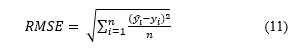
3.5. Root Mean Square Error (RMSE)

The standard deviation of the residuals is defined as the Root Mean Square Error (RMSE) or otherwise known as prediction errors. Residuals are a measure of how far away the data points are from the regression line; RMSE is a measure of how spread out these residuals are. In other words, it indicates how concentrated the data is near the line of best fit. The root mean square error is a term that is frequently used in climatology, forecasting, and regression analysis.

4. Results and Discussion

The data we are using is secondary data obtained from hargapangan.id, id.investing.com, and Bank Indonesia website, the data are from August 2017 until March 2020. We are going to use two data sets, rice price data set and egg price data set. Each of the datasets contains the national and regional (DKI Jakarta) food commodity price (e.g.: rice price and egg price), USD buying price against IDR, and Gold price. In this research, all independent variables are used in predicting the food commodity price in DKI Jakarta. The independent variables are dependent on time.

The variables above are the national food price, USD buying price against IDR, and gold price, which is represented by x1, x2, x3, and time represented by t.

The data analyzed has different units, so it is necessary to have a data center and scale for standardization of each variable. The standardization is done using Z-Score normalization.

Table 1: Normalized Rice Price Data Set

No	X1 (t-1)	X2 (t-1)	X3 (t-1)	X1(t)	X2(t)	X3(t)	Y(t)
1	-0.946	-1.473	-0.630	-0.948	-1.468	-0.639	-0.149
2	-0.946	-1.475	-0.638	-0.978	-1.480	-0.679	-0.149
3	-0.976	-1.487	-0.678	-0.978	-1.480	-0.779	-0.280
…	…	…	…	…	…	…	…
970	1.076	4.225	2.447	1.074	4.388	2.382	1.393

Table 2: Normalized Egg Price Data Set

No	X1 (t-1)	X2 (t-1)	X3 (t-1)	X1(t)	X2(t)	X3(t)	Y(t)
1	-2.524	-1.473	-0.630	-2.535	-1.468	-0.639	-2.388
2	-2.524	-1.475	-0.638	-2.535	-1.480	-0.679	-2.388
3	-2.524	-1.487	-0.678	-2.535	-1.480	-0.779	-2.388
…	…	…	…	…	…	…	…
970	0.458	4.225	2.447	0.226	4.388	2.382	0.886

We first calculated the VIF score for each independent variable, in a linear regression model, the result can be found in table 3.

Table 3: VIF linear regression model using rice data set

Independent Variables	VIF
X1(t-1)	4.4681
X2(t-1)	108.432
X3(t-1)	39.536
X1(t)	4.4394
X2(t)	113.610
X3(t)	40.553

From table 3 we could see that there is high multicollinearity in a few variables mainly X₂ and X₃ which are the USD buying value against IDR and gold price.

Table 4: VIF ridge regression model using rice data set

Independent Variables	VIF
X1(t-1)	0.329
X2(t-1)	0.156
X3(t-1)	0.198
X1(t)	0.329
X2(t)	0.157
X3(t)	0.195

After applying the data into a ridge regression model, the VIF value decreases significantly (VIF<5). This proves that ridge regression can deal with multicollinearity problems found in linear regression. Using the proposed method for multiple linear regression and ridge regression in section 3 for our model, we get the prediction results in figure 1 and figure 2.

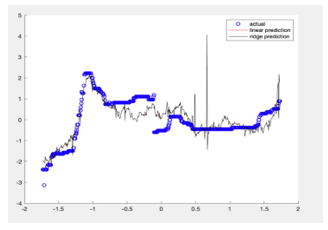Figure 1: Linear Regression and Ridge Regression with the best damping factor prediction using Rice Price data set

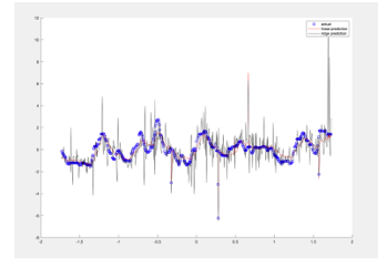Figure 2: Linear Regression and Ridge Regression with the best damping factor prediction using Egg Price data set

Based on figure 1, we could see that the prediction using ridge regression is closer to the actual line. In table 5 and table 6 we compare the performance of each model.

Table 5: Performance Overview using Rice Price Dataset

	RMSE	MAPE	Computational Time
Linear Regression (cross-validation)	0.7461	-0.0157	1.558560s
Ridge Regression (cross-validation)	0.6062	-0.2568	0.938901s
ANFIS Model	56.3763	0.0019672	52 s
Linear Regression (with the best damping factor)	0.04510	0.0421578	0.162167s
Ridge Regression (with the best damping factor)	0.04510	0.0421577	0. 228641s

Table 6: Performance Overview using Egg Price Dataset

	RMSE	MAPE	Computational Time
Linear Regression (cross-validation)	0.5557	0.0471	1.680529 s
Ridge Regression (cross-validation)	0.5329	0.1062	0.936147 s
ANFIS Model	474.4033	0.0063840	58s
Linear Regression (with the best damping factor)	0.03622	0.03548663	0.231017 s
Ridge Regression (with the best damping factor)	0.03622	0.03548587	0.175020 s

From the performance in Table 5 and 6, in rice dataset the proposed RR model performs good with 4,2% MAPE evaluation, but it is still higher compared the ANFIS model which shows 0,19 % of MAPE evaluation. While the MAPE value in LR and RR model using CV turns out to be negative in value. This might be caused by the particular small actual values that could bias the MAPE, and how in some cases the MAPE implies only which forecast is proportionally better In the egg data set where the proposed RR model performs in average 3,5% MAPE, better than the one using Cross Validation, but it is still higher compared to ANFIS which have an MAPE score of 0,63%. If we compared the computational time, the regression model performs in a much faster speed compared to the cross-validation model and the ANFIS model where the proposed RR model in average could compute in less than a second while ANFIS model took almost a minute to generate the results. This is because the training time that are usually used to find the optimal results could be reduced by finding the damping factor firsthand.

5. Tables and Figures

This study demonstrated how a ridge regression model can be used as an effective way to forecast the food price prediction in DKI Jakarta. These models acquired accuracy in food prediction, on the model where we had to calculate the ridge parameter/damping factor beforehand also shows a faster computation time compared to the one where we used cross-validation.

The proposed model uses a linear ridge regression equation by [20], a future study using a different equation should be done to improve the overall performance. Since the dataset we are using is fairly small (970 (t) observation), using a bigger data set may show a more significant computational time difference. Further study by using a nonlinear forecasting model or implementing the kernel method should be to enhance the current model so it could produce better results.

Conflict of Interest

The authors declare no conflict of interest.

Acknowledgment

The Authors thank Bina Nusantara University for supporting this research.

1. FAO, How to Feed the World in 2050, 2012.
2. BPS, Rata-Rata Konsumsi per Kapita Seminggu Beberapa Macam Bahan Makanan Penting, 2007-2018, 2018.
3. X. Lin, H. Liu, P. Lin, M. Wang, “Data mining for forecasting the broiler price using wavelet transform,” Journal of Convergence Information Technology, 5(3), 113–121, 2010, doi:10.4156/jcit.vol5.issue3.16.
4. L. Bayari, S.K. Tayebi, “A Prediction of The Iran’s Chicken Price by the ANN and Time Series Methods,” Agricultural Economics Department, 1–12, 2008.
5. D. Bhuriya, G. Kaushal, A. Sharma, U. Singh, “Stock market predication using a linear regression,” Proceedings of the International Conference on Electronics, Communication and Aerospace Technology, ICECA 2017, 2017-Janua, 510–513, 2017, doi:10.1109/ICECA.2017.8212716.
6. H.F. Zou, G.P. Xia, F.T. Yang, H.Y. Wang, “An investigation and comparison of artificial neural network and time series models for Chinese food grain price forecasting,” Neurocomputing, 70(16–18), 2913–2923, 2007, doi:10.1016/j.neucom.2007.01.009.
7. A.G. Assaf, M. Tsionas, A. Tasiopoulos, “Diagnosing and correcting the effects of multicollinearity: Bayesian implications of ridge regression,” Tourism Management, 71(September 2018), 1–8, 2019, doi:10.1016/j.tourman.2018.09.008.
8. M.A. Rasyidi, “Prediksi Harga Bahan Pokok Nasional Jangka Pendek Menggunakan ARIMA,” Journal of Information Systems Engineering and Business Intelligence, 3(2), 107, 2017, doi:10.20473/jisebi.3.2.107-112.
9. A.R. Tanjung, Z. Rustam, “Implementasi Regresi Ridge dan Regresi Kernel Ridge dalam Memprediksi Harga Saham Berbasis Indikator Teknis,” 2013.
10. M. Ali, R. Prasad, Y. Xiang, R.C. Deo, “Near real-time significant wave height forecasting with hybridized multiple linear regression algorithms,” Renewable and Sustainable Energy Reviews, 132(September 2019), 110003, 2020, doi:10.1016/j.rser.2020.110003.
11. G.L. Baird, S.L. Bieber, “The goldilocks dilemma: Impacts of multicollinearity-A comparison of simple linear regression, multiple regression, and ordered variable regression models,” Journal of Modern Applied Statistical Methods, 15(1), 332–357, 2016, doi:10.22237/jmasm/1462076220.
12. J.D. Kasarda, “multicollinearity (highly,” 5(4), 461–470, 1977.
13. J.M. Herrera, L.L. Häner, A. Holzkämper, D. Pellet, “Evaluation of ridge regression for country-wide prediction of genotype-specific grain yields of wheat,” Agricultural and Forest Meteorology, 252(October 2017), 1–9, 2018, doi:10.1016/j.agrformet.2017.12.263.
14. A.S. Goldberger, “Best Linear Unbiased Prediction in the Generalized Linear Regression Model,” Journal of the American Statistical Association, 57(298), 369–375, 1962, doi:10.1080/01621459.1962.10480665.
15. C.G.U. and G.N. Amahis, “Comparative analysis of rainfall prediction using statistical neural network and classical linear regression model.pdf,” Journal of Modern Mathematics and Statistics, 5(3), 66–70, 2011, doi:10.3923/jmmstat.2011.66.70.
16. B.M. Golam Kibria, A.F. Lukman, “A new ridge-type estimator for the linear regression model: Simulations and applications,” Scientifica, 2020, 2020, doi:10.1155/2020/9758378.
17. A.E. Hoerl, “Application of ridge analysis to regression problems,” Chemical Engineering Progress Symposium Series, 58, 54–59, 1962.
18. A.E. Hoerl, R.W. Kennard, “On regression analysis and biased estimation,” Technometrics, 10, 422–423, 1968.
19. A.E. Hoerl, “Ridge Analysis,” Chemical Engineering Progress Symposium Series, 60, 67–77, 1964.
20. A.E. Hoerl, R.W. Kennard, “Ridge Regression: Biased Estimation for Nonorthogonal Problems,” Technometrics, 1970, doi:10.1080/00401706.1970.10488634.
21. A.E. Eoerl, R.W. Kaanard, K.F. Baldwin, “Ridge Regression: Some Simulations,” Communications in Statistics, 4(2), 105–123, 1975, doi:10.1080/03610927508827232.
22. M. Goldstein, S. Chatterjee, B. Price, “Regression Analysis by Example.,” Journal of the Royal Statistical Society. Series A (General), 1979, doi:10.2307/2982566.
23. G. Bollinger, D.A. Belsley, E. Kuh, R.E. Welsch, “Regression Diagnostics: Identifying Influential Data and Sources of Collinearity,” Journal of Marketing Research, 1981, doi:10.2307/3150985.
24. R.M. O’Brien, “A caution regarding rules of thumb for variance inflation factors,” Quality and Quantity, 2007, doi:10.1007/s11135-006-9018-6.
25. T.A. Craney, J.G. Surles, “Model-dependent variance inflation factor cutoff values,” Quality Engineering, 2002, doi:10.1081/QEN-120001878.

(Click Here)