Application of Piecewise Linear Approximation of the UAV Trajectory for Adaptive Routing in FANET

Volume 6, Issue 2, Page No 559-565, 2021

Author’s Name: Kuzichkin Oleg R.^1,a), Vasilyev Gleb S.¹, Surzhik Dmitry I.², Kurilov Igor A.²

^a)Author to whom correspondence should be addressed. E-mail: oldolkuz@yandex.ru

Adv. Sci. Technol. Eng. Syst. J. 6(2), 559-565 (2021);   DOI: 10.25046/aj060263

Keywords: Unmanned aerial vehicle, UAVs, Flying Ad Hoc Network, FANET, Routing, Trajectory approximation, Piecewise linear function

1. Introduction

This paper is an extension of work originally presented in the 7th International Conference on Control, Decision and Information Technologies (CoDIT’ 20) [1]”.

Networks built on the basis of unmanned aerial vehicles (UAVs) (Flying Ad Hoc Network, FANET) [2] are characterized by an unstable network topology due to the movement of network nodes. This aspect should be taken into account when developing and applying routing algorithms. The well-known network layer protocols do not fully meet the requirements of the FANET, so the development of new routing protocols for flying networks remains relevant.

Proactive protocols calculate routes between all network nodes beforehand and maintain a relevant routing table at each node [3]. An integral part of such routing protocols is a connection management mechanism that establishes logical connections between network nodes that are within earshot of each other, and also closes logical connections. All stations distribute information about the established logical connections over the network. Thus, each of the stations decentralizes the logical topology of the network and fills in its own routing table. In addition, proactive routing protocols provide minimal delay in the delivery of data packets, and when the network topology changes, broadcast messages about these changes are initiated [4].

The author proposed a reactive protocol Dynamic Source Routing (DSR) [5]. In reactive routing protocols, routes exist only when they are needed, that is, when data is being transmitted over them. When the route is initially determined, packets are sent in all possible directions, and information about the passed node is added to the header. As a result, when the goal is reached, the packet header contains a fully formed route between the specified nodes. In the event of loops, i.e. re-reception of the first packet, the node destroys this packet. The high mobility of FANET nodes when using proactive protocols requires frequent updates of the routing table, which is their disadvantage.

Hybrid routing protocols combine the advantages of reactive and proactive routing protocols, but require a relatively complex implementation. Their use is associated with the need to divide the network structure into segments, which reduces the efficiency of routing (for example, HWMP-Hybrid Wireless Mesh Protocol).).

Geographic routing protocols use the spatial coordinates of network nodes and are more efficient for FANET, especially when the network is large. An example is the Greedy Perimeter Stateless Routing protocol (GPSR) [6]. Directional antennas-based protocols reduce the number of transit nodes and, as a result, lower the delay time (DOLSR-Directional Optimized Link State Routing Protocol [7]).

A significant problem of routing protocols in the Flying Ad Hoc Networks (FANET) is a significant overhead cost due to the high mobility of networking nodes. The problem is caused by a need to send information messages between nodes about locations of separate unmanned aerial vehicles (UAVs) [8]. Also the use of directional antennas on board the UAV [9-11] necessitates additional transmition of the angular coordinates of each node, since when the airplane turns, the receiving antenna may deviate from the maximum of the radiation pattern, which will reduce the useful signal.

In [1] the application of UAV trajectory approximation for adaptive routing in FANET networks is justified. However, the expressions are given in a fairly brief form. In addition, the approximation example of a trajectory fragment in the form of a sinusoidal function does not allow us to fully evaluate the advantages of the proposed approach, for which it is necessary to model a trajectory consisting of a set of straight sections and curved sections with variable steepness.

2. The algorithm for conjugated courses

Approximation of the UAV trajectory will reduce the overhead caused by the transmission of additional information about the position of network nodes. The use of trajectory approximation algorithms will allow the vehicle coordinates to be transmitted only at the beginning or end of each maneuver. With this approach, it is not necessary to transmit data about intermediate points of the trajectory between maneuvers, which reduces overhead costs.

The creation of the trajectory of an flying vehicle consists of several stages [12]. The first is to set the motion kinematics, which determines the spatial position of the object at an arbitrary time t. For this purpose, the object is assigned a trajectory that can be set by a set of reference vertices with a velocity vector defined at each vertex. Next, the trajectory of the air object is plotted along the reference verteces. The main disadvantage of the method of conjugating courses is a rather large amount of calculations and, accordingly, a decrease in the speed of the algorithm.

The course matching algorithm is based on dividing the trajectory into segments, and each segment is described as a mathematical expression [13]. The input data of the algorithm are the coordinates of the node points of the trajectory. The rectilinear motion of the aircraft is described by parametric equations:

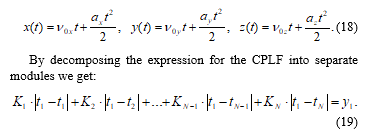
where x and y are current spacial coordinates, x₀ and y₀ are initial values of spacial coordinates, are projections of velocity on x and y axis, a_x and a_y are projections of acceleration on x and y axis, accordingly.

When calculating straight segments of the trajectory, the minimum trajectory curvature radius with a nominal (acceptable) level of overload, it is necessary to calculate the coefficient

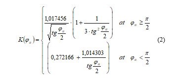where φ_n is course at the segment n of a trajectory.

For circular segments of the trajectory, when calculating speed, one might need to calculate the sine, cosine:

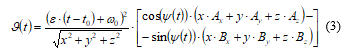where  is current radial velocity of an aircraft, ε is circular acceleration, t and t₀ is current and initial time, ω₀ is initial circular velocity, x, y, and z are spatial coordinates, ψ is current current manuevering angle, A_x,y,z and B_x,y,z are coefficients of the movement.

For parabolic segments when calculating the maximum move in a parabola, there is a need also calculate the arc sine:

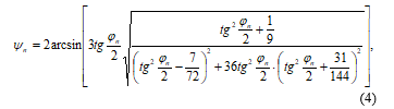where ψ_n and φ_n are current manuevering angle and course at the segment n of a trajectory.

Expressions (1-4) describe a smooth trajectory with high accuracy, which is necessary in automatic control systems [14] and simulation systems of full-scale modeling of aircraft [12, 15]. However, routing algorithms do not require such high accuracy in describing the path. The main requirement for the routing algorithm is the choice of optimal transit nodes for a specific network topology, which can be successfully performed with small errors in the representation of the trajectory. Thus, for routing algorithms the very detailed trajectory model is redundant, computationary complex and not required.

3. Algorithms based on continuous piecewise linear functions

Studies have shown that continuous piecewise linear functions (CPLF) based on the modulus of a linear function are effective for approximating nonlinear characteristics, trajectories [16-18]. Calculating the approximation coefficients and the function itself requires less computational resources compared to the course conjugation algorithm.

A smaller value of the error is achieved at the expense of equality of error in every area of approximation. The use of this approach when approximating straight lines leads to a decrease in the error, since the approximating function “adjusts” (adapts) to the change in the nature of the nonlinearity of the original characteristic.

The approximation of the trajectory using the adaptive CPLF is schematically shown in Figure 1. The function section is divided into segments. The approximation nodes are calculated as follows: a fixed error value is set, then the number of segments (approximation nodes) is determined by the algorithm. The length of segment xi varies depending on the value of approximation error ε.

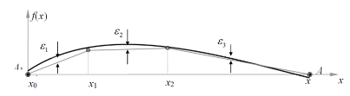Figure 1: The principle of trajectory approximation using CPLF

The CPLF approximation assumes the replacement of the object’s trajectory along an arc with the trajectory of movement along a straight line. The time and velocity modules are selected according to the reference algorithm [12]. As a result, in both cases (trajectories  and ) start and end speed is the same and time spent is also the same. This means that each point of the reference segment is projected onto the corresponding point of the CPLF segment. For example, consider a section of the trajectory of Figure 1 in the interval [x₀, x₁]. It is shown in Figure 2. It can be seen that the error in determining the position of the object on the segment is equal to the maximum length of the projection line. In the adaptive CPLF, the errors  are aligned with each other. The geometric meaning is shown in Figure 3.

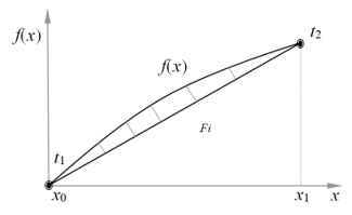Figure 2: Fragment of the trajectory

The actual error is the distance between the position of the object on the reference curve and its position on the approximating curve. Figure 3 shows the discrepancy between the actual error and the approximation error. Knowing that  we estimate the range of changes in the error value . From the right triangle ABC in Figure 4, we obtain , where  is the angle between the CPLF and the reference trajectory. Thus

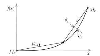Figure 3: Determination of the approximation error

To estimate the error  we need to know the error . The minimum value  (at the origin in Figure 4), The maximum value  and , therefore the actual error  is determined by the inequalities  and  It follows from the inequality that the greater the value of φ, the smaller the error , and  (the side of the triangle ABC) does not exceed . This means that  is the maximum error of the approximation of the reference trajectory using the CPLF.

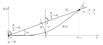Figure 4: Determination of the linear and angular approximation error

3.1. Basic CPLF

It has a compact form and contains only one approximation coefficient. The basic CPLF is convenient for representing functions and nonlinear characteristics approximated with a fixed argument step, with a small number of approximation nodes. The base CPLF has the form:

where  is an initial shift of the CPLF relative to the origin;

Δt is a shift of the modules relatively to each other;

M=0,1,2,3 is a count of the number of modules;

 is approximation coefficient.

Summing up the four functions shifted relative to each other by a fixed value, we get the basic CPLF (Figure 5):

We determine the coefficients . To do this, using the four points ; ; ;  shown in the figure, we make a system of four equations:

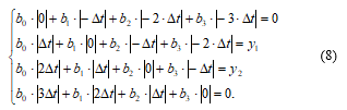After the transformations, the system takes the form:

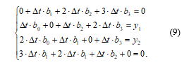Solving system (9) by the Gauss method [20], we obtain:

where  are the function values in the approximation nodes.

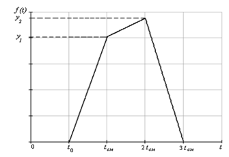Figure 5: Basic CPLF

In order not to use separate expressions for each coefficient , we present them as a single coefficient :

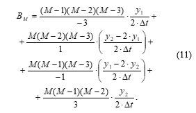We transform equation (11):

Substituting the coefficient , we finally get:

The disadvantages of the basic CPLF include a cumbersome expression for determining the approximation coefficients . In addition, to approximate functions over a large number of points (more than three), it is necessary to add up individual base CPLFS shifted between each other.

3.2. Generalized CPLF

The generalized CPLF reduces the computational cost of approximation using the basic CPLF. This function is the sum of a few basic CPLF. Using the generalized CPLF, we can approximate functions of any kind based on a single expression for the approximating function, rather than a large number of expressions:

where  is the approximation coefficient, n is the number of basic CPLF for the approximation; is the initial offset of the second approximating function;  are values of the initial characteristic in odd approximation nodes;

 are values of the initial characteristic in even approximation nodes.

The disadvantages of the generalized CPLF include additional terms under the module and two sum counters, which complicates the computational process. A generalized CPLF can have a compact notation form and include only one sign of the sum.

3.3. Generalized CPLF with compact notation

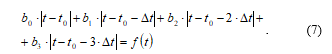
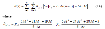
We design a function that has a compact expression and allows us to perform an approximation with an arbitrary step. It is the sum of the modules of linear functions with different coefficients in front of them. Expressions under modules represent shifts of linear functions in the time domain. These shifts determine the approximation step. Thus, shifting the individual linear functions by a different value t_n we get the CPLF:

where n is the sum counter; t_n is the approximation step; K_n is the approximation coefficient.

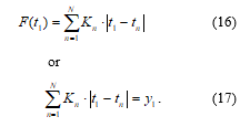
We define an expression for finding the coefficient K_n. To do this, we approximate the function  using  points. Let the first approximation node correspond to the value , and the value of the approximated function . The expression for the CPLF at this point:

The law of motion along each straight segment can be given by a function of the parameter t:

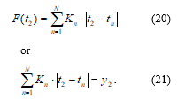
We perform a similar operation for the second node , which corresponds to the value of the approximated function  and the expression for the adaptive CPLF at this node:

As a result, for N approximation nodes we obtain a system of N equations:

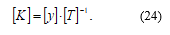
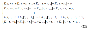We find the values of the coefficients K₁ – K_N by the inverse matrix method. In matrix form, the system will take the form:

Hence, the desired coefficients K₁ – K_N have the form:

3.4. Adaptive CPLF

Approximating trajectories with a fixed step is impractical if the trajectories contain long straight sections. To represent each linear fragment, two approximation points are sufficient, and it is advisable to place most of the approximation points on curved sections. Thus, it is promising to apply an adaptive CPLF with a variable approximation step.

As a criterion for the quality of the approximation, we use the minimum mean square error (MSE) criterion. The expression for the approximation MSE in the range (t₀, t_N) has the form

The approximation is carried out based on finding the vector T = (t₁ … t_N–1)^T which fits to the condition of the mimumum MSE value:

Adaptive CPLF allows to approximate nonlinear characteristics and functions with a lower error than CPLF with a fixed approximation step. This is achieved by obtaining an equal error in each approximation section. The use of this approach when approximating with lines leads to a decrease in the error, since the approximating function “adjusts” (adapts) to the change in the nature of the nonlinearity of the original characteristic.

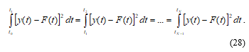
Equal approximation error in each section will reduce the total error. To obtain an equal approximation error in each section, the following condition must be met:

Based on the MSE expressed by Equation (25), we write:

Let’s represent the integrand expressed in Equation (28) as follows:

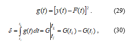where G is antiderivative of the function g(t).

We find the points for the approximation of an arbitrary function based on the adaptive CPLF with a lower error. To find these points, we define a system of equations:

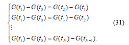From the system of equations (31), the values of t_n are determined, which approximate the studied characteristic with an equal error in each section. The values of the function y(t_n) at the points t_n are determined from the known expression for the original function y (t).

4. Approximation of the trajectory fragment of the aircraft based on the CPLF

The solution of the minimization problem (26) was performed on the basis of the nonlinear conjugate gradient method [19,20], the value of convergence tolerance parameter of 10^–6 was accepted. Evaluation of the approximation MSE based on Equation (25) is shown in Fig. 3.

The approximation result of the aircraft trajectory fragment _1,2(t) by N=16 nodes and the absolute approximation error D_F1,2(t) are shown in Figures 6 and 7. Here, the lower index 1 corresponds to the uniform law for the approximation nodes, and the index 2 corresponds to the optimal law. The dots in the figures show the approximation nodes. The values of the source function and the approximating function at the nodes are equal, so the error at these points is zero. The MSE values are s²_F1=1,187×10^–3; s²_F2=1,982×10^–5. With the optimal nodes, most of them are located on a curved section, where the trajectory changes most quickly, which gives a significant decrease of MSE (by 59.9 times).

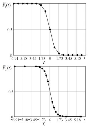Figure 6: Approximation of the aircraft trajectory fragment based on the CPLF: a) with a uniform step; b) with an adaptive step

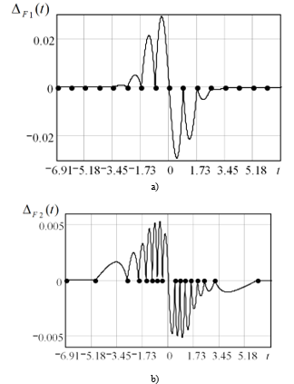Figure 7: Approximation error of the aircraft trajectory fragment based on the CPLF: a) with a uniform step; b) with an adaptive step

5. Modeling of approximation-based routing in FANET

A comparative simulation of the UAV network with two routing protocols was performed: the standard ad-hoc on-demand vector (AODV) and the modified one. In the modified version of the protocol, Route Request packets were not transmitted at a fixed time interval, as in the standard version, but only when the course changed by more than 200. Otherwise, Route Request packets were not transmitted, and the coordinates of the nodes obtained from the past coordinate values by the piecewise linear approximation were used to update the route table. Changes in the course of individual nodes were taken into account in the node mobility model (the OPNET modeler 14.5 simulator was used). Thus, the modified routing protocol is a hybrid of the standard AODV protocol and geographic-based routing. When modeling the network, the following parameters were obtained:

• the number of network nodes – 20;
• channel bandwidth – 2 Mbit/s;
• the power of the UAV receiving and transmitting device is 10 mW;
• threshold receiving power-minus 90 dB;
• the maximum data packet size is 1024 bytes;
• MAC layer protocol – CSMA/CA (carrier sense multiple access with collision avoidance)
• network size 10×10 km;
• average speed of mobile nodes is 10 m/s.

Mobility model – Random-Waypoint [21]

During the simulation, the Pause time parameter of a mobility model (time between changes in direction and/or speed) was varied and the routing overhead in percent was determined for the standard and modified AODV. The simulation results are shown in Figure 8. The overhead value of the standard AODV is in good agreement with the results in [22]. The modified version of AODV routing protocol shows a lower overhead value (the gain for small pause time values reaches 23 %). Thus, the effectiveness of the proposed approximation-based routing in FANET is shown.

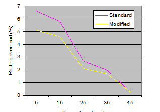Figure 8: Routing overhead vs Pause time for a standard and modified AODV

6. Conclusion

A serious problem of routing protocols in FANET is the significant overhead caused by the high mobility of network nodes. The problem is caused by a need to send information messages about locations of unmanned aerial vehicles (UAVs). The perspective of algorithms for constructing the UAV trajectory to reduce the amount of service information about the UAV position transmitted via the FANET routing protocols is substantiated. When using such algorithms, information about the coordinates of the nodes is directly transmitted only in the areas of maneuvering of the aircraft, and in the areas of rectilinear motion is calculated based on the algorithms for approximating the trajectory. In order to reduce the amount of service information, the following trajectory approximation algorithms have been investigated: an algorithm for conjugating courses and an algorithm based on continuous piecewise-linear functions (CPLF). Four modifications of the CPLF algorithm are considered which differ in the type of function used: basic CPLF, generalized CPLF, generalized CPLF with a compact notation form, and adaptive CPLF. The advantages and disadvantages of each algorithm are analyzed. Adaptive CPLF with variable approximation step allows lower computational resources compared to the rate-matching algorithm, as well as more accurate compared to the CPLF with a fixed step.

An approximation of a trajectory fragment consisting of two straight sections and a curved section with a variable steepness between them (approximately described by the arctangensoidal function) was performed. The computational experiment has shown the effectiveness of the direct approach: in the considered example with long straight sections, the approximation MSE by the adaptive CPLF is 59.9 times less compared to the fixed step CPLF. The modified version of ADV routing protocol shows a lower overhead value (the gain for small pause time values reaches 23 %). Thus, the effectiveness of the proposed approximation-based routing in FANET is shown.

Acknowledgment

The work was supported by the RFBR grant 19-29-06030-mk “Research and development of a wireless ad-hoc network technology between UAVs and smart city control centers based on the adaptation of transmission mode parameters at various levels of network interaction”. The theory was prepared within the framework of the state task of the Russian Federation FZWG-2020-0029 “Development of theoretical foundations for building information and analytical support for telecommunications systems for geoecological monitoring of natural resources in agriculture”.