1. Introduction

This work is an extension based originally on the groundwork presented in the 4th IEEE Sciences and Humanities International Research Conference (SHIRCON-2019) [1]. This paper will focus on the improvements of the mechanical, electronic and electrical design, as well as the implementation of the Q-Learning algorithm while Ref. [1] focuses on the preliminary design of the vehicle, the development of the vision algorithms to be used and the development structure in the simulation environment.

Obstacle detection and avoidance in autonomous vehicles is mandatory for these smart systems to work fully. To the present, there are multiple algorithms of imminent detection and evasion developed by the automotive industry with a really appreciable rate of precision. Thus, in order to get closer to achieving these results, it is essential that the mechanical, electronic and electrical design of the vehicle has specific criteria in the most important considerations that are related to the objective of detection and evasion. That is why, for example, the design of the steering system must provide the closest modeling to reality, in order to obtain the best parameters to include in the simulation environment. On the other hand, for the overall vehicle design to respond according to the results obtained in the simulation, the electronic and electrical design must take into account the appropriate selection of components, as well as their interaction.

Consequently, Figure 1 shows the final design of the vehicle. Despite the changes made, the safety factor has maintained its value of 1.8, this is because when considering the improvements, the distribution of mass which allowed the most critical areas to be subjected to less stress.

For the additional calculus in the present paper, the approximate value of power of the vehicle is 1911 watts. The mechanical efficiency is 96%, effective power of approximately 2000 watts is required. According to the previously obtained value of power, a 2.5 HP PCM motor was selected for the impulse of the vehicle, this motor has a maximum speed of 2800 RPM. Additionally, another motor appointed to control the car’s steering system was required. For this case, a 350 watts DC motor was selected.

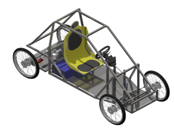Figure 1: Isometric view of the 3D model of the chassis and components.

With the details described above, they allowed the previous research to obtain a preliminary mechanical, electronic and electrical design based on the considerations of making a low-cost prototype. Likewise, the baselines for the recognition of the environment that will allow the artificial intelligence algorithm to be trained. However, the design in general had not been developed in depth and in detail on the most relevant considerations for the intelligent algorithm, such as the vehicle’s turning design and the brake system, as well as its integration into the electronic and electrical design.

This research has the following outline: Section 2 will introduce the improved vehicle’s mechanical design. Next, the improved vehicle’s electronic and electrical design is presented in Section 3. Then, Section 4 will present the Q-Learning algorithm results. Finally, Section 5 will discuss the conclusion of the findings.

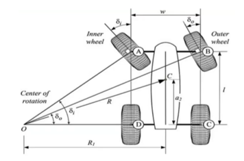Figure 2: Ackerman Principle [2]

2. Mechanical Design Enhancement

2.1. Steering System

The direction of a vehicle is responsible for orienting some or all of its wheels so that it takes the desired path. It was found that for a better turning behavior, in the case of a four-wheel vehicle with its steering system on the front axle, it is necessary for the inner wheel to turn a greater angle than the outer one, because the inner wheel follows a smaller turning radius than the outer wheel. It was also found that to experience even better turning behavior, the projections of the axes perpendicular to the steering axle of the wheels must intersect at the same point. This behavior is called the Ackerman principle, after Rudolph Ackerman patented it in 1817 for use in horse carts [2]. The Ackerman Principle is shown in the following figure.

To guarantee a close point of rotation of both wheels, which ensures almost zero skid angles at low speeds when the vehicle goes around a curve, the Ackerman configuration shown in by the following expression.

                                   cot(??) – cot(??) = ?/?                              (1)

Where ?? is the steering angle of the outer wheel, ?? is the steering angle of the inner wheel, ? is the distance between the axes of the wheels, called Track, and ? is the distance between the front and rear axles of the vehicle, called Wheelbase, as shown in the figure [2].

In the same way, an expression can be obtained that describes the radius of gyration of the center of mass of the vehicle in steady state. This is calculated by the following expression.

                                      R² = ?2² + ?²cot²(?)                                 (2)

Where ?2 is the distance on the vehicle’s axis of travel between the rear axle and the center of mass and ? is the cotangent average of the internal and external angles of the wheels.

Therefore, to determine the closeness of a mechanism to the behavior of the Ackerman configuration, an error function must be determined, in this manner by minimizing its value, get the closest expected result according to the configuration that was found. This function can be expressed as a mean square error (RMS) value. In this case, the error function cannot be explicitly defined and must be evaluated for ? values of the mentioned angles. The expression that determines the mean square error value of a set of discrete values of ?r is defined by the following equation [3].

                               er² =                           (3)

Where ??? is the angle of the external wheel of the developed mechanism and ??? is the angle of the external wheel of the Ackerman configuration according to the characteristics of the vehicle for a range of internal wheel angles ?? determined.

The drawback in this case is to be able to determine the external wheel angle ?? for an internal wheel angle value ?? in a given mechanism. Showers and Lee present in their document “Design of the Steering System of an SELU Mini Baja Car” a methodology to determine internal and external wheel angles for a steering mechanism used corresponding to that of a Daewoo Damas model car [4].

Finally, according to the proposed mechanical design, there is a value of ? equal to 0.994 meters and a value of ? equal to 1.960 meters, as well as a value of ?2 approximately 0.784 meters, for which when performing the iterations in MATLAB, it was obtained that the radius of gyration R corresponds to a value of 0.803 meters, which is within the established limits.

2.2. Braking System

The principle of a braking system is the reduction of kinetic and potential energy that a vehicle presents when it is in motion. This energy is transformed into heat energy and is dissipated in the brake discs, produced by the friction of the brake pads. Therefore, to select a component that meets the vehicle’s requirements, it is necessary to find the maximum torque provided [5]. A figure illustrating this is shown below.

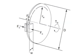Figure 3: Brake Disc Diagram [5]

where Fc is the clamping force of the brake mechanism and re is the effective radius. The braking torque is calculated by the following expression.

                                         T = 2(Fc)(re)(u)                                    (4)

According to the selected braking system, there is a value of Fc equal to 1000 Newton and a value of re equal to 0.09 meters, as well as a value of u, coefficient of friction, approximately 0.2, with these values it was obtained that the braking torque T corresponds to a value of 36 Newton-meters. On the other hand, the maximum torque generated by the vehicle’s engine is equivalent to a value of around 32 Newton-meters. This value is the result of the chain drive reduction used; the ratio of 15 teeth on the pinion and 72 teeth on the spur gear, delivers 1:4.8, which equates to a maximum speed of approximately 583 RPM. Therefore, this torque value is less than the brake system torque.

3. Electronic and Electrical Design Enhancement

The electronic and electrical enhancement of this electric vehicle (EV) is focused in two main critical points. First, safety features like anti-lock brake system (ABS) and traction control system (TCS) were added. Second, mandatory equipment like head lights, direction indicator lights and others were considered in the design. In addition, electronic controls and better understanding of the connections are reviewed.

3.1. Anti-lock Brake System and Traction Control System

The simplest anti-lock brake and traction control systems are based on the information acquired through speed sensors that are placed in each wheel. Both of them may use this information to control and stabilize the vehicle by assuring that the wheels are spinning as intended.

The ABS prevents the brakes from locking up the wheels. It maintains the steerability and controllability of the vehicle under braking circumstances [6]. The electronic control unit (ECU) receives the information of the speed sensors and performs control techniques in order to regulate the brake pressure applied on the pedal. Figure 4 shows a common ABS control loop of an internal combustion engine (ICE) vehicle.

The TCS prevents the wheels from overspinning. It maintains the stability and traction when accelerating [7]. In this case, the ECU receives the same information as the ABS, but, depending on the design, TCS may have two variants. On one hand, the TCS with brake intervention activates the brakes of the overspinning wheels until they match the speed of the other ones. On the other hand, the TCS with engine intervention reduces the amount of power the overspinning wheels are receiving until they match the speed of the other ones. A comparison is shown in Figure 5.

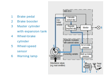Figure 4: ABS control loop [7]

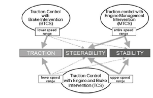Figure 5: TCS variants comparisons [8]

These systems are tested in different types of environments and scenarios. For example, a vehicle equipped with ABS and TCS must not lose control on certain types of surfaces (e.g. wet surface), must be stable during acceleration or braking and must deal with curves without losing traction. Apart from that, it is important to know that these systems should be calibrated according to the vehicle itself because parameters like the torque of the motor or the size of the wheels may change its dynamics, thus the control algorithm for these systems.

For this work, ABS and TCS with engine intervention are included in the vehicle’s design as safety features. They are meant to be simple, effective and complementary. The objective is to increase the variety of environments and scenarios the vehicle is capable to deal with.

The connection diagram of the EV is presented to have a better understanding of the vehicle’s internal distribution (see Figure 6). The main components are the 2000 watts’ permanent magnet synchronous motor (PMSM), the motor controller, the 72 V lead-acid battery pack, the gear shift lever, the ignition key, the brake and the throttle. These components are enough to make the EV move forward or backward. In addition, two DC-DC converters are necessary. On one hand, a 72 V to 12 V converter is used to power other components that run on 12 V and later on 5 V for the microcontroller or sensors. On the other hand, a 72 V to 24 V converter is used to power the steering motor.

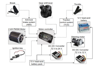Figure 6: EV connection diagram

The throttle and the brake are different from each other. On one hand, the throttle uses hall sensors to measure its position. It is powered with 5V and delivers a signal from 1 V to 4.8 V into the throttle pin of the motor controller when manipulated. On the other hand, the brake is a simple switch that connects 12 V to the brake pin of the motor controller (electric brake). The ABS and TCS concept for this design relies on activating or deactivating the throttle and the brake when necessary. For this purpose, a window comparator circuit is implemented in Arduino and simulated in Proteus (see Figure 7).

The main components used for the simulation are the Arduino MEGA with ATmega 2560 microcontroller, the IRF9530 MOSFET transistor and the 2N3904 BJT transistor. The input signals are attached to the interrupt pins (18, 19 and 20) of the microcontroller so it doesn’t miss any data while sensing. These signals simulate the speed sensors (Hall effect sensors). LED D1 and LED D2 represent the throttle and the brake (ON state means enabled and OFF state means disabled). It is important to notice that the ABS and TCS can be activated or deactivated depending on the user’s decision. The user only needs to close the switch to bypass any of those systems.

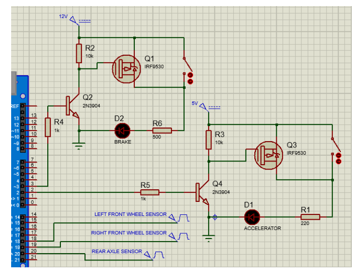Figure 7: ABS and TCS simulation

The speed sensor used for the design is the A1104 Hall effect sensor (see Figure 8). Two are placed in the front wheels and one is placed on the rear axle. This sensor will commute when detecting the south pole of the magnetic ring (48 north poles and 48 south poles) attached to the rotary axles of each wheel. The time is measured between each pulse and compared with each sensor to determine if the wheels are locked up or overspinning. First, if the wheels lock up while braking, the microcontroller deactivates the brake (ABS) but keeps the throttle activated. Second, if the wheels start overspinning, the throttle is deactivated (TCS) but keeps the brake activated. Third, if the speed of each wheel is almost equal, no control is applied and both remain activated. A difference threshold is considered for the simulation in case the sensors do not match properly. For TCS a threshold of 5 RPM to 10 RPM was estimated and for ABS a threshold of 30 RPM or higher was considered. These values may vary depending on the road conditions and the level of the systems’ effectiveness. They must be calibrated based on that information.

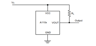Figure 8: Schematic of the A1104 sensor [9]

The following calculations were made to assure a correct behavior of the device. The A1104 sensor has a slew rate of 2.5 V/us and it works on 5 V. This gives a 2 us rise and fall time for this voltage. It means that the signal could have a period four times the rise time, in other words, a frequency of 125 kHz before it gets distorted. The maximum speed of the motor reaches 5000 RPM (84 Hz) without load and with flux weakening. As mentioned before, there are 48 south poles that will trigger the sensor and gives a maximum frequency of 4032 Hz. This frequency is far below the 125 kHz and determines that will work properly. The complete connection diagram is showed in Figure 9.

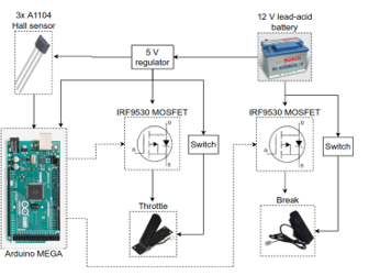Figure 9: ABS and TCS connection diagram

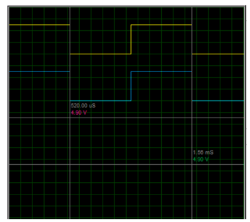Figure 10: Normal state

The results can be seen in Figure 10, Figure 11 and Figure 12 (Proteus’ oscilloscope). The yellow signal represents the left front wheel sensor (only using one as a reference), the blue signal represents the rear axle sensor, the red signal controls the activation of the break and the green signal controls the activation of the throttle. First, Figure 10 shows a normal state in which both sensors match the same frequency. This means that the wheels are spinning at the same speed and no control is applied. The break and the throttle are activated (4.90 V and 4.90 V respectively). Second, Figure 11 shows an overspinning situation in which the rear axle sensor is measuring a higher frequency than the front wheel sensor. This means that the rear wheels are spinning faster than the front wheels. The brake remains activated and the throttle is deactivated (4.90 V and 0 V respectively). Third, Figure 12 shows a lock up situation in which the rear axle sensor is measuring a lower frequency than the front wheel sensor. This means that the rear wheels are spinning slower than the front wheels. The brake is deactivated and the throttle remains activated (0 V and 4.90 V respectively).

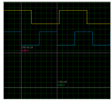Figure 11: Overspinning situation

Figure 12: Lock up situation

3.2. Equipment

All vehicles are enforced to follow certain specifications in their design to be admitted to circulate on the streets. Minimum requirements include head, reverse, indicator and brake lights. These lights were included in the design and are graded to be used on almost any vehicle (see Figure 13). White reverse lights are activated with the gear shift lever, red brake lights are activated if the head lights switch is closed or the brake is applied, and amber indicator lights, head lights and the cabin light are activated with a switch.

This vehicle is powered by six 12 V lead-acid batteries connected in series (total of 72 V) and a 12 V lead-acid battery for the electronics, accessories and other equipment. Each battery has 55 Ah of capacity and the total energy of the vehicle is estimated to be 330 Ah or 4 kWh (including the six pack only). Eventually, the batteries will lose energy when being used and will need to be recharged. In this case, a commercial 72 V charger and a solar charging system is being included in the design (see Figure 14).

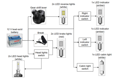Figure 13: Lights connection diagram

The charger itself is capable of delivering 12 A, so it will take approximately 30 hours to completely charge the vehicle. It is recommended not to discharge these batteries below 40% of their capacity because they could be damaged and decrease their performance.

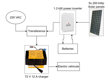Figure 14: Charging infrastructure

The solar charging system is calculated based on a full charge for the EV assuming that it won’t be discharged below 40% (4 kWh*0.6 = 2.4 kWh). All the parameters for this system are obtained with the software Stringsizer from ABB and it will be considered On the grid (Lima, Peru). The peak sun hour (PSH) is determined considering the mean during a year in Lima and is equal to 5.71 kWh/m². The performance ratio (PR) is a constant value applied to give a margin in case more energy is required and is equal to 0.8. The kilo Watt-hour (kWh per day) is the amount of energy needed, for this design, it is considered to be 2.4 kWh that was calculated previously. The following expression is used to establish the power needed for the solar panels.

                                    kWh = (kWp)(HSP)(K)                              (5)

After making the calculations, the results determine that a 0.52 kWp (kilo Watt peak) solar charging system is required. Considering a 2 m² and 200 Wp solar panel, the system requires a minimum of 3 solar panels. To increase the efficiency due to inverters, a group of 5 panels with a total of 1.2 kWp and a 1.2 kW power inverter are chosen. A battery bank with the same vehicle’s capacity is recommended but not essential.

4. Applied Intelligence

Reinforcement learning (RL) is defined as a sequential decision-making problem of an agent that has to learn how to perform a task through trial and error interactions with an unknown environment which provides feedback in terms of numerical reward [10,11].

The Markov process is the theoretical basis of reinforcement learning, which can be expressed by the Q-learning algorithm, which is the most classical and commonly used algorithm to solve the MDP problem. It can only be used to solve MDP problems with actions and state spaces both discrete and finite. With an initial Q-table and a predefined policy, in each step, the agent selects an action based on the current state, which according to the reward is fed back and the observation of the next state, the Q table is updated using the algorithm described in the section 4.1, to finally repeat the steps until the Q function converges to an acceptable level [12].

With the Q Learning algorithm, we can allow intelligent agents to operate in environments with discrete action spaces. The discrete action space refers to actions that are well defined, such as movement from left to right, up or down.

For example, in the context of autonomous driving, while the dynamics of the autonomous vehicle is clearly a Markov decision process, the next state depends on the behavior of other elements such as vehicles, pedestrians or cyclists, which are not necessarily an MDP [13].

Therefore, in the case of the design proposed as a starting point for local research in our region, it is convenient to dispense with those elements that are not MDP. Thus, in the context of autonomous driving, given the unpredictable behavior of vehicles or pedestrians, these elements will not be considered for the reinforcement learning algorithm.

4.1. Algorithm

We start by defining the appropriate set of desires for driving based on the desired speed of the vehicle and the angle of rotation that the turn allows. On the other hand, a cost function is needed on the conduction paths that corresponds to its location by means of coordinates in a plane. The cost that is assigned to a trajectory corresponds to the weighted sum of the individual cost assigned to the speed and position. Additionally, weights are assigned to each of the costs described above to obtain a single objective function to control the trajectory. Therefore, the policy consists of a mapping of the state of desires and a mapping of the requested trajectory. This last mapping is implemented by solving an optimization problem whose cost depends on the set of desires [14].

Algorithm 1: Q-Learning
function: Q-Learning Agent (percept) returns an action
Initialization; inputs: percept, indicating the current state s’ and reward r’ persistent: Q, a table of action values indexed by state and action, initially zero Nsa, a table of frequencies for state-actions pairs, initially zero s, a, r, the previous state, action and reward, initially null
if Terminal?  (s) then Q[s, none] ← r’
	if s is not null then
		Increment Nsa[s, a] Q[s, a] ← Q[s, a] + alpha(Nsa[s, a])(r + y Q[s’, a’]- Q[s, a]) s, a, r  ← s’, argmax((Q[s’, a’]- Q[s, a]),Nsa[s’, a’]), r’
return a

The Q values correspond to the utility of executing each action a in state s, that is, the action of advancing or stopping in a state of object detection, as well as the action of evading by turning in a state mentioned above. Also, alpha and y are the hyper parameters for tuning the algorithm.

4.2. Results

During the development of the algorithm in the GAZEBO simulation environment, it was important that the algorithm be able to calculate the “road parameters”, these correspond mainly to the speed of the vehicle, which includes acceleration or deceleration, and the steering angle.

After having tried different rates of learning, no great progress has been made. This is because the optimal local solution could be due to the magnitude gap between the reward value and the punishment, leading to a large number of training epochs. on the way. Finally, the learning procedure converges after approximately 250 episodes. The vehicle can evade fixed obstacles by avoiding sudden changes in acceleration by means of a speed and angle of turn.

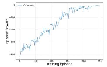Figure 15: The evaluation of the algorithm

The figures below show the implementation of the model in the simulation environment together with objects that can be detected by the LIDAR sensor and the camera. Figure 16 shows how the vehicle with the sensor region and camera field of view, Figure 17 shows its interaction with the environment and Figure 18 and 19 shows the decision and evasion sequence to avoid colliding with an object.

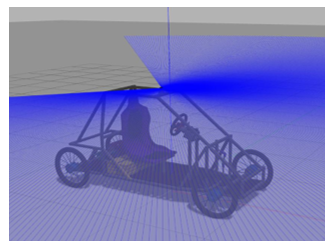Figure 16: Implementation of the 3D model in the simulated environment

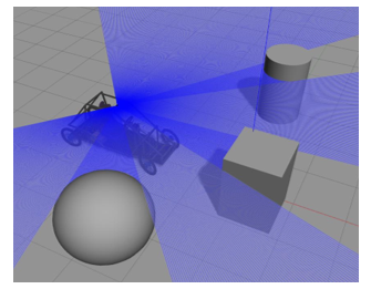Figure 17: Interaction of vehicle with the environment

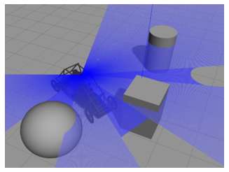Figure 18: Actions of the vehicle with the environment

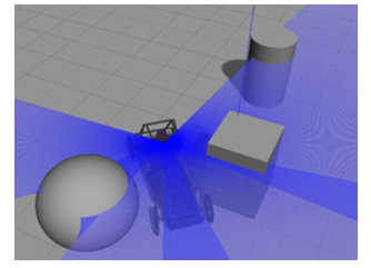Figure 19: Actions of the vehicle with the environment

5. Conclusions

It was achieved that the mechanical design, taking into account the manufacturing and budget limitations, is based on the methodologies for the correct operation of the system in general such as the steering system. On the other hand, design improvements will be analyzed and developed according to the completion of manufacturing. It is appropriate to mention that, as a consequence of the pandemic that has been affecting the world population, the implementation and manufacture of the vehicle has been stopped to safeguard the health of the members.

The electronic and electrical design enhancement has proved its benefits. First, safety on road has increased due to the addition of the anti-lock brake and traction control systems. The simulations determined the effectiveness of the control algorithm design for this vehicle. This algorithm was aimed to work better on wet surfaces, but it was not simulated for other kinds of terrain, like mud or gravel. It enhanced the driver response and the stability of the vehicle. Second, mandatory equipment has been added to allow the circulation of this vehicle on the streets. This also increased safety while driving among other vehicles. A future insertion to the cities automotive fleet is closer. Finally, an EV has a low carbon footprint in comparisons to the ICE vehicles. To keep this track, a solar charging system demonstrated that it is not necessary to utilize the city power, mostly if this energy is generated by hydrocarbons.

Finally, the classical Q-learning algorithm is unfeasible for more complex control problems, since each additional dimension contributes exponentially to the size of the state space, with it a significant high-dimensional preprocessing. Thus, there are other techniques such as DDPG, which combines the DQN algorithm, Deterministic Policy Gradient (DPG) and Actor-Critic [15]. The basic idea consists of the repetition of experiences to eliminate relevance, since at the moment of storing the experiences of an agent and then randomly extracting batches to train a neural network, a more solid learning for the specific tasks can be guaranteed. For example, the results obtained by Chen, Seff, Kornhauser and Xiao use the algorithm described above as a baseline, and show the penalties it gets and the large amount of processing required to reach an optimal policy (around 80,000 iterations) [16]. However, the proposal of this paper includes simplifications in the mechanical and electrical design that allow reducing the dimensionality of the Q-learning algorithm, which results in a much faster dimensional processing and penalties close to 0 compared to the DDPG algorithm. Therefore, the best driving parameters according to the proposed vehicle design are obtained by the Q-learning algorithm. The subsequent optimization will be the training with controlled situations implemented in the simulation environment, such as street generation and route indication. In this way, once the prototype has finished its manufacture, perform the integration with ROS so that the simulation environment allows the agent to obtain the actions closest to a real situation.

Conflict of Interest

The authors declare no conflict of interest.

Acknowledgment

This implementation was funded by IEEE RAS Chapter Initiative Grants and by Faculty of Sciences and Engineering of the Pontifical Catholic University of Peru.

1. J. Valera, L. Huaman, L. Pasapera, E. Prada, L. Soto, L. Agapito, “Design of an autonomous electric single-seat vehicle based on environment recognition algorithms,” 2019 IEEE Sciences and Humanities International Research Conference (SHIRCON), 1–4, 2019, doi:10.1109/SHIRCON48091.2019.9024852.
2. H. Heiser, Vehicle and Engine Technology, 2nd ed., Society of Automotive Engineers, 1999.
3. R.N. Jazar, Vehicle Dynamics: Theory and Application, 2nd ed., Springer-Verlag New York, 2014, doi:10.1007/978-1-4614-8544-5.
4. A. Showers, H.-H. Lee, “Design of the Steering System of an SELU Mini Baja Car,” International Journal of Engineering Research & Technology (IJERT), 2(10), 2396–2400, 2013.
5. G. Rill, Road Vehicle Dynamics: Fundamentals and Modeling, 1st ed., CRC Press, 2012.
6. K. Reif, ed., Brakes, Brake Control and Driver Assistance Systems: Function, Regulation and Components, 1st ed., Springer Vieweg, 2014, doi:10.1007/978-3-658-03978-3.
7. K. Reif, ed., Fundamentals of Automotive and Engine Technology: Standard Drives, Hybrid Drives, Brakes, Safety Systems, 1st ed., Springer Vieweg, 2014, doi:10.1007/978-3-658-03972-1.
8. B. Heißing, M. Ersoy, eds., Chassis Handbook: Fundamentals, Driving Dynamics, Components, Mechatronics, Perspectives, 1st ed., Vieweg+Teubner Verlag, 2011, doi:10.1007/978-3-8348-9789-3.
9. Allergo, Continuous-Time Switch Family A110X, 1–11, 2012.
10. S. Russell, P. Norvig, Artificial Intelligence: A Modern Approach, 4th ed., Pearson, 2020.
11. H.J. Vishnukumar, B. Butting, C. Müller, E. Sax, “Machine learning and deep neural network — Artificial intelligence core for lab and real-world test and validation for ADAS and autonomous vehicles: AI for efficient and quality test and validation,” 2017 Intelligent Systems Conference (IntelliSys), 714–721, 2017, doi:10.1109/IntelliSys.2017.8324372.
12. C.J.C.H. Watkins, Learning from Delayed Rewards (PhD. thesis), University of Cambridge, 1989.
13. L. Wang, N. Zhang, H. Du, “Real-time identification of vehicle motion-modes using neural networks,” Mechanical Systems and Signal Processing, 50–51, 632–645, 2015, doi:10.1016/j.ymssp.2014.05.043.
14. N. van Hoorn, J. Togelius, D. Wierstra, J. Schmidhuber, “Robust player imitation using multiobjective evolution,” 2009 IEEE Congress on Evolutionary Computation, 652–659, 2009, doi:10.1109/CEC.2009.4983007.
15. T.P. Lilicrap, J.J. Hunt, A. Pritzel, N. Heess, T. Erez, Y. Tassa, D. Silver, D. Wierstra, “Continuous control with deep reinforcement learning,” 4th International Conference on Learning Representations (ICLR), 1–14, 2016.
16. C. Chen, A. Seff, A. Kornhauser, J. Xiao, “DeepDriving: Learning Affordance for Direct Perception in Autonomous Driving,” 2015 IEEE International Conference on Computer Vision (ICCV), 2722–2730, doi:10.1109/ICCV.2015.312.

(Click Here)