1. Introduction

In today’s economy, gold is becoming an essential financial commodity. Gold has become the underlying value for many reasons. Security is the first one. Gold is a robust investment instrument, capable of preserving its liquidity even in crises such as political turbulence [1] and the COVID-19 pandemic [2].              The second is that when they have had problems with their balance of payments, many nations have repeatedly used gold collateral against loans. The final reason is that for coping with inflation, gold will serve as a guide. Research on gold’s value is fundamental because gold prices can quite directly reflect the economy’s market expectations. Gold value prediction is a difficult task, primarily because of the unusual shifts in economic patterns and, on the other hand, insufficient knowledge. ARIMA is a classical approach focused on the estimation of statistical time series and a prediction model for univariate time series. The critical drawback of ARIMA is the model’s pre-assumed linear shape. With the rise of machine learning, artificial neural networks in time series forecasting have been widely studied and used.

Recurrent neural networks (RNN) [3] are often seen as the most efficient time series prediction method. RNN is a subset of artificial neural networks in which nodes are connected in a loop, and the internal state of the network can exhibit dynamic timing behavior. However, as the length of the processing time series increases, problems such as gradient disappearance often occur during the training of RNNs using conventional activation functions, such as tanh or sigmoid functions, limiting the prediction accuracy of the RNN. According to Ahmed & Bahador, the highest precision RNN is LSTM (Long Short Term Memory) Neural Network[4]. LSTM has an outstanding efficiency in natural language processing, while this model can also solve long-term dependencies very well. Since problems with long-term dependencies exist in the prediction of time series, researchers are trying to use LSTM to solve problems with time series, such as forecasting of foreign exchange [5, 6], traffic flow analysis [7, 8], and gold ETF[9]. The Gated Recurrent Unit is another type of RNN (GRU). GRU is an RNN-based network, a form of gated RNNs, which largely mitigates the gradient vanishing problem of RNNs through gating mechanism and make the structure simpler while maintaining the effect of LSTM [10]. This research’s main objective is to study RNN forecasting methods that offer the best predictions for multivariate gold price prediction concerning lower forecast errors and higher accuracy of forecasts. Research on multivariate analysis has multiple features to determine the predicted value.

The dataset for the prediction model consists of eight features after feature selection is  conducted :

1. Gold Price in IDR
2. Gold Price in USD
3. Gold Price in Euro
4. Gold Price in GBP
5. Gold Price in RMB
6. Jakarta Stock Exchange Composite (IHSG)
7. Hang Seng Index
8. NASDAQ Composite Index

Historical data on this paper is gathered from the World Gold Council website (gold.org) and investing.com. Data is collected in an interval of 20 years, start from 2001 to 2020. The author split the dataset into 70% training data and 30% testing data. The validation data is a subset of training data, and the length is 10% of the total data. The validation data is based on 20 years dataset.

2. Literature Review

2.1. Data Preprocessing

Pre-processing is a method to develop data to form good shape for data training. Data pre-processing is a fundamental stage of the machine learning application, which has been reported to significantly impact the performances of machine learning methods [11]. Data pre-processing techniques include reduction, projection, and missing data techniques (MDTs). Data reduction decreases the data size via, for example, feature selection (FS) or dimension reduction [12].

2.2. Grid Search

Grid search is a process that attempts each hyper-parameter combination extensively and selects the best as the optimal hyper-parameters[13]. The grid search method is theoretically capable of finding optimal solutions. However, it suffers from severe limitations in the following aspects. It can not provide optimal solutions within a sufficient reach with limited computational resources. However, Grid search specializes in addressing discrete hyper-parameters [14].

2.3. Feature Selection

Feature selection is referred to as obtaining a subset from an original feature set by selecting the dataset’s relevant features according to the unique feature selection criteria [15]. Feature selection has a vital role in compressing the data processing size, where the redundant and irrelevant characteristics are eliminated. Feature selection techniques can pre-process learning algorithms, and proper feature selection results can improve learning accuracy, reduce learning time, and simplify learning results [16].

2.4. Long Short Term Memory (LSTM)

Long short-term memory (LSTM) is an altered version of RNN proposed to learn long-range dependencies across time-varying patterns [17]. Generally, LSTM is a second-order recurrent neural network that solves the vanishing and exploding gradients issue by replacing RNN simple units with the memory blocks in a recurrent hidden layer. A memory cell is a complex processing unit in LSTM with many units shown in Figure 1.

It comprises one or many memory cells, adaptive multiplicative gating units (input, output, and forget), and a self-recurrent connection with a fixed weight of 1.0. It serves as a short-term memory with control from adaptive multiplicative gating units. The input and output flow of a cell activation of a memory cell is controlled by input and output gate, respectively. Forget gate was included in memory cell [18] that helps to forget or reset their previous state information when it is inappropriate.

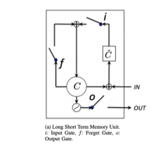Figure 1: LSTM Cell Unit: Image Source [19]

2.5. Gated Recurrent Unit (GRU)

The GRU is a simpler derivative of the LSTM network, and in some cases, both produce comparative results. Although there are major similarities in architecture for the purpose of solving vanishing gradient problems, there are several differences. The structure of a GRU module is shown in Figure 2.

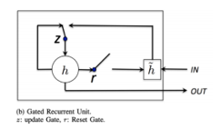Figure 2: GRU Cell Unit: Image Source [19]

The GRU cell does not have a separate memory cell-like LSTM cell architecture, according to [20]. In addition to having three gating layers like LSTM in each module, the GRU network only has two gating layers, a reset gate, and an update gate. The reset gate decides how much information to forget from the previous memory. The update gate acts similar to the forget and input gate of an LSTM cell. It decides how much information from previous memory can be passed along to the future.

3. Methodology

3.1. Data Collection and Preprocessing

This research collects gold price values on a daily basis. The collected data has twelve features: gold price in Indonesian Rupiah (IDR), gold price in US Dollar (USD), gold price in Euro (Euro), gold price in Pound sterling (GBP), gold price in Chinese Renminbi (RMB), gold to silver ratio, Japanese Stock Market Index (Nikkei 225), Indonesian Stock Composite Index (IHSG), Shanghai Hang Seng Index (Hang Seng), Nasdaq Index (Nasdaq), US Dollar and Indonesian Rupiah currency pair (USD/IDR), Australian Dollar and US Dollar currency pair (AUD/USD). The price and supporting data were collected from January 1, 2001, to 09:00 on December 31, 2020, through the World Gold Council (gold.org) and investing.com.

Table 1: Example of the collected raw gold price data

Date	IDR	USD	Euro	GBP	RMB	Gold / Silver	Nikkei 225	IHSG	Hang Seng	Nasdaq	USD/IDR	AUD/USD
Dec 22 2020	26664206.89	1877.1	1542.6	1409.6	12290.9	73.41	26436.39	6023.29	26119.25	12717.56	14145.0	0.7521
Dec 23 2020	26625000.00	1875.0	1538.6	1386.7	12258.4	73.27	26524.79	6008.71	26343.1	12653.14	14150.0	0.7572
Dec 28 2020	26540625.00	1875.0	1535.1	1394.6	12257.8	71.09	26854.03	6093.55	26314.63	12838.86	14140.0	0.7577
Dec 29 2020	26483859.69	1874.3	1531.1	1389.3	12240.1	71.78	27568.15	6036.17	26568.49	12843.49	14110.0	0.7605

Table 2: Feature Correlation Value towards IDR

Features	Correlation Coefficient Value	Is Removed
IDR	1.000000	No
USD	0.924278	No
Euro	0.969419	No
GBP	0.970746	No
RMB	0.932027	No
Gold/Silver	0.467344	Yes
Nikkei 225	0.627255	Yes
IHSG	0.924860	No
Hang Seng	0.798830	No
Nasdaq	0.868520	No
USD / IDR	0.776257	No
AUD / USD	0.301990	Yes

Table 3: Pre-processed gold data for the raw data of Table 1

Date	IDR	USD	Euro	GBP	RMB	IHSG	Hang Seng	Nasdaq	USD/IDR
Dec 22 2020	26664206.89	1877.1	1542.6	1409.6	12290.9	6023.29	26119.25	12717.56	14145.0
Dec 23 2020	26625000.00	1875.0	1538.6	1386.7	12258.4	6008.71	26343.1	12653.14	14150.0
Dec 28 2020	26540625.00	1875.0	1535.1	1394.6	12257.8	6093.55	26314.63	12838.86	14140.0

3.2. Feature Selection

Feature selection is implemented by calculating Pearson’s Correlation Coefficient. The correlation value can be seen in Table 2, and the visualization of feature correlation could be inferred in Figure 3.

The defined threshold for features correlation is 0.75. All features that have correlation coefficient values below the threshold would be removed, and all features above that point will be used as selected features. An example of pre-processed data can be seen in Table 3.

3.3. Model Training and Validation

The prediction in this work is to utilize the LSTM model to forecast the gold price. As a modified version of the recurrent neural network model, the LSTM model [21] defines whether the weight value is maintained by adding cell states in an LSTM cell.

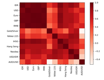Figure 3: Pearson Correlation Matrix of All Features

The LSTM model can accept an arbitrary length of inputs, and it can be implemented flexibly and in various ways as required. The state obtained from an LSTM cell is used as input to the next LSTM cell, so the state of an LSTM cell affects the operation of the subsequent cells. The LSTM predictive model has the capability to remove or add information to the LSTM cell state.

The information that enters the cell is controlled by gates, a component that represents a way to save or forget information through the LSTM cell unit.

In order to enrich and benchmark the proposed LSTM model, this research also develops a GRU prediction model. GRU model is similar to LSTM and is known to have good forecasting performance for a shorter time period.  The same model tuning process for the GRU prediction model was also performed for the purpose of fairness. The overall training and tuning process is summarized in Figure 4.

3.4. Hyperparameter Tuning

Hyperparameter optimization is an essential step in the implementation of any machine learning model [22]. This optimization process includes regularly modifying the model’s hyperparameter values to minimize the testing error. Based on research, kernel initializer and batch size rate need to optimize for better accuracy [22]. Meanwhile, the author proposed dropout rate, neuron units, and learning optimizer [23]. Research from Google Brain Scientist studied the relation between two hyperparameters, batch size, and learning rate [24]. When the learning rate is decay, random fluctuation appears in the SGD dynamics. Instead of decaying the learning rate, that research increase the batch size. That strategy achieves near-identical model performance on the test set with the same number of training epochs but significantly fewer parameter updates. However, when the batch size is large, this often causes instabilities during the early stages of training. In consequence, the optimum batch size value must be decided for the best prediction result.

Furthermore, the dropout rate indicates the fraction of the hidden units to be dropped to transform the recurrent state in the LSTM layer. Finally, the optimization type designates the optimization algorithm to tune the internal model parameters to minimize the cross-entropy loss function [23]. This paper combines two prior research and choose the batch size, kernel initializer, dropout rate, neuron units, and learning optimizer based on the references. The proposed hyperparameter candidates for LSTM could be shown in Table 4 and GRU in Table 5.

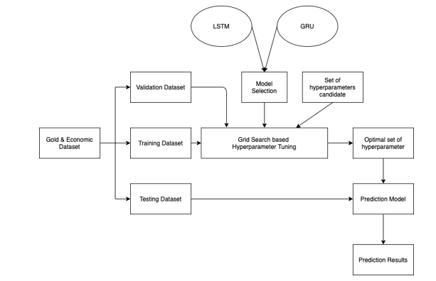Figure 4: Prediction model training and tuning process with grid search

The kernel initializer represents the strategy for initializing the LSTM and Dense layers weight values. The activation type represents the activation function that produces non-linear and limited output signals inside the LSTM, Dense I, and II layers.

Table 4: Candidate and optimal sets of hyper-parameters for LSTM

Hyper-parameter name	Hyper-parameter values candidate	Optimal Hyper-parameter values
Kernel Initializer	lecun_uniform, zero, ones, glorot_normal, glorot_uniform, he_normal, he_uniform, uniform, normal, orthogonal, constant, random_normal, random_uniform	ones
Batch Size	16, 32, 64, 128, 256, 512, 1024	16
Dropout Rate	0.0, 0.2, 0.3, 0.4	0.0
Neuron Units	32, 64, 128	128
Learning Optimizer	SGD, RMSProp, Adagrad, Adam	Adam

Table 5 : Candidate and optimal sets of hyper-parameters for GRU

Hyper-parameter name	Hyper-parameter values candidate	Optimal Hyper-parameter values
Kernel Initializer	lecun_uniform, zero, ones, glorot_normal, glorot_uniform, he_normal, he_uniform, uniform, normal, orthogonal, constant, random_normal, random_uniform	ones
Batch Size	16, 32, 64, 128, 256, 512, 1024	64
Dropout Rate	0.0, 0.2, 0.3, 0.4	0.0
Neuron Units	32, 64, 128	64
Learning Optimizer	SGD, RMSProp, Adagrad, Adam	Adam

3.5. Model Evaluation

In order to measure the error of the prediction model for the time series problem, the researcher utilizes Root Mean Squared Error (RMSE) and Mean Absolute Percentage Error (MAPE).

3.5.1. Root Mean Squared Error

Root Mean Squared Error (RMSE) is derived from Mean Squared Error. It represents the average difference between predicted and real value. The formula of RMSE can be seen in (1). RMSE is common practice to calculate the accuracy of the prediction model.

3.5.2. Mean Absolute Percentage Error

Mean Absolute Percentage Error (MAPE) calculates the average delta between predicted and real value and represent in percentage. The formula of MAPE can be seen in (2).

4. Results and Analysis

4.1. Prediction Result for Simple LSTM and GRU

Table 6 shows the training result of the proposed methods and some state of arts who have studied a forecasting gold price model. Inspire by that state of arts, the author utilizes RMSE and MAPE to evaluate the proposed model. The proposed models have 25 epochs, 32 batch sizes, a 0.2 dropout rate value, 32 neuron units, a uniform kernel initializer, and RMSProps Learning Optimizer. Derive from Table 6 can be known that GRU has lower error for three months until three years than LSTM. For the period above three years, LSTM has a lower error rate.

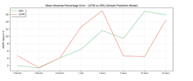Figure 6: MAPE Value of Simple Prediction Model

Table 6: Forecasting Result with Simple Prediction Model

Simple Prediction Model
Interval	RMSE		MAPE
	LSTM	GRU	LSTM	GRU
3 Months	1,305,470.42	628,984.55	4.68 %	1.96 %
4 Months	476,750.72	460,679.94	1.40 %	1.30 %
6 Months	1,260,382.60	1,262,250.99	4.07 %	4.07 %
1 Year	3,529,122.74	1,813,811.23	12.57 %	6.43 %
3 Years	4,528,491.45	3,043,471.50	17.02 %	11.61 %
5 Years	1,012,206.71	2,164,846.99	4.61 %	9.40 %
10 Years	983,174.32	3,276,504.50	4.46 %	16.89 %
20 Years	2,784,692.49	3,055,371.13	14.43 %	15.90 %

As presented in Figure 5, the value of RMSE for both LSTM and GRU is decreased over time. However, GRU has a lower error rate in intervals until three years, while LSTM is more accurate in the above three years intervals. RMSE indicates the average value of the difference between the predicted and real value.

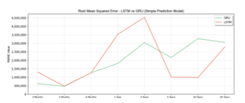Figure 5: RMSE Value of Simple Prediction Model

As presented in Figure 6, the value of MAPE for both LSTM and GRU is decreased over time. However, GRU has a lower error rate in intervals until three years, while LSTM is more accurate in the above three years intervals. MAPE indicates the percentage of the overall delta between predicted and real value.

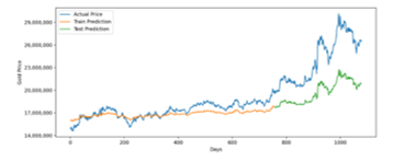Figure 7: LSTM Prediction for 3 Years Training Data

LSTM prediction model for three years period is accurate in train prediction but moderately inaccurate in test prediction, as seen in Figure 7. Averagely, it has around 4 million rupiah difference between predicted and real value that represented by RMSE. The reason is LSTM needs a large dataset to predict accurately.

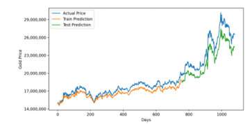Figure 8: GRU Prediction for 3 Years Training Data

On the contrary, for three years period, the GRU model gives good accuracy. Averagely, it has around 3 million rupiah difference between predicted and real value that represented by RMSE. It indicates that, for intervals up to 3 years, the GRU model is preferable.

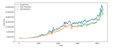Figure 9: LSTM Prediction for 20 Years Training Data

Figure 9 shown the LSTM prediction model for twenty years period. The model has pretty good accuracy. Averagely, it has around 2.7 million rupiah difference between predicted and real value that represented by RMSE.

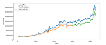Figure 10: GRU Prediction for 20 Years Training Data

For twenty years period, the GRU model slightly less accurate than the LSTM model. Averagely, it has around 3 million rupiah difference between predicted and real value that represented by RMSE. It indicates that, for intervals up to 20 years, it is better to use the LSTM model. According to data in Table 6, LSTM accuracy increase over time, while GRU accuracy is great for a short time period but has lower accuracy for a long period. However, the accuracy can be improved by applying Hyperparameter Tuning using Cross Validated Grid Search.

Table 7: Forecasting Result with Grid Search Optimized Prediction Model

Grid Search Optimized Prediction Model
Interval	RMSE		MAPE
	LSTM	GRU	LSTM	GRU
3 Months	905,316.59	1,878,634.45	3.25 %	7.12 %
4 Months	379,823.43	1,486,398.71	0.97 %	5.52 %
6 Months	336,076.94	1,348,307.28	0.87 %	4.82 %
1 Year	415,606.27	384,696.30	1.06 %	1.00 %
3 Years	354,942.67	343,101.59	0.96 %	0.94 %
5 Years	314,599.02	278,038.93	0.90 %	0.77 %
10 Years	227,230.62	232,294.05	0.74 %	0.76 %
20 Years	213,036.85	216,012.48	0.72 %	0.73 %

4.2. Prediction Result for Optimized LSTM and GRU

Model Optimization for LSTM and GRU conducted by applying Hyperparameter tuning using Cross Validated Grid Search. Grid Search tries every value on the hyperparameter candidate that is stated in Table 4 for LSTM and Table 5 for GRU.  After Grid Search was conducted, the best result for each iteration becomes hyperparameter value on Optimized LSTM and GRU Model. The optimized LSTM models have 25 epochs, 16 batch sizes, a 0 dropout rate value, 128 neuron units, “ones” kernel initializer, and utilize ADAM optimizer. The training result of optimized LSTM and GRU using grid search based hyperparameter tuning can be seen in Table 7. Derive from Table 7, and it can be known that for three months until three years, GRU has lower error than LSTM. For the period above three years, LSTM has a lower error rate. Results accuracy of the optimized model can be seen in Figure 11 for RMSE and Figure 12 for MAPE.

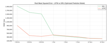Figure 11: RMSE Value of Optimized Prediction Model

Figure 11 shows that in the optimized model, LSTM has a better RMSE score than GRU in almost all time intervals. GRU model slightly performs better in time interval one year until three years.

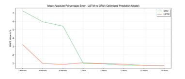Figure 12: MAPE Value of Optimized Prediction Model

Figure 12 also shows a similar result with RMSE. MAPE score in the optimized model, LSTM has better accuracy than GRU in almost all time intervals. GRU model also slightly performs better in time interval one year until three years. It indicates that, for the model that is optimized with grid search, LSTM has better accuracy than the GRU predicted model.

Forecasting gold price for three years interval using optimized LSTM and GRU model has a similar result. It has a 354942.67 RMSE value for LSTM and 343101.59 for GRU. In MAPE measurement, LSTM has 0.96 error, while GRU has 0.96 error. It indicates that for interval three years, GRU Model is slightly more accurate.

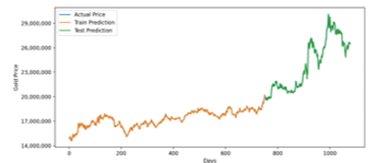Figure 13: Optimized LSTM Prediction for 3 Years Training Data

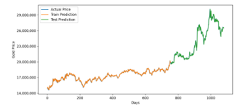Figure 14: Optimized GRU Prediction for 3 Years Training Data

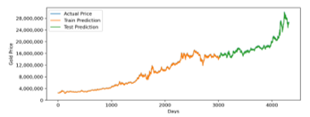Figure 15: Optimized LSTM Prediction for 20 Years Training Data

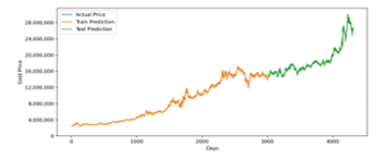Figure 16: Optimized GRU Prediction for 20 Years Training Data

Forecasting gold price for twenty years intervals using optimized LSTM and GRU model also has a similar result. It has a 213036.85 RMSE value for LSTM and 216012.48 for GRU. In MAPE measurement, LSTM has 0.72 error, while GRU has 0.73 error. It indicates that for the interval of twenty years, LSTM Model is slightly more accurate. Summary prediction result accuracy for all time intervals can be seen in Table 8.

5. Conclusion

According to the training, validation, and hyperparameter tuning, the best model to use in gold price forecasting problems for time intervals under three years period is GRU. On the other hand, for time intervals above three years, LSTM is shown higher accuracy. That is shown by RMSE and MAPE Score. Grid Search based Hyperparameter tuning is proven to increase LSTM accuracy significantly by decreasing its error. Table 8 shows that

Table 8: Prediction Model Forecasting Result Summary

RMSE							MAPE
Interval	LSTM			GRU			LSTM			GRU
	Simple	Optimized	Delta	Simple	Optimized	Delta	Simple	Optimized	Delta	Simple	Optimized	Delta
3 Months	1,305,470.42	905,316.59	31%	628,984.55	1,878,634.45	-199%	4.68%	3.25%	1,43%	1.96%	7.12%	-5,16%
4 Months	476,750.72	379,823.43	20%	460,679.94	1,486,398.71	-223%	1.40%	0.97%	0,43%	1.30%	5.52%	-4,22%
6 Months	1,260,382.60	336,076.94	73%	1,262,250.99	1,348,307.28	-7%	4.07%	0.87%	3,2%	4.07%	4.82%	-0,75%
1 Year	3,529,122.74	415,606.27	88%	1,813,811.23	384,696.30	79%	12.57%	1.06%	11,51%	6.43%	1.00%	5,43%
3 Years	4,528,491.45	354,942.67	92%	3,043,471.50	343,101.59	89%	17.02%	0.96%	16,06%	11.61%	0.94%	10,67%
5 Years	1,012,206.71	314,599.02	69%	2,164,846.99	278,038.93	87%	4.61%	0.90%	3,71%	9.40%	0.77%	8,63%
10 Years	983,174.32	227,230.62	77%	3,276,504.50	232,294.05	93%	4.46%	0.74%	3,72%	16.89%	0.76%	16,13%
20 Years	2,784,692.49	213,036.85	92%	3,055,371.13	216,012.48	93%	14.43%	0.72%	13,71%	15.90%	0.73%	15,17%
Average			68%	Average		2%	Average		6,72%	Average		5,74%

grid search can averagely decrease 68% RMSE and decrease 6,72 MAPE score. It also improves GRU Model, averagely decreases RMSE by 2%, and decreases 5,74 MAPE score. From that information, this research shows that hyperparameter tuning is more effective in optimizing LSTM Model than GRU Model for this research, gold price prediction problem. For future research, it is good to apply metaheuristic methods, such as Ant Colony Optimization, Genetic Algorithm, or Chaotic Metaheuristic, to conduct hyperparameter tuning with better performance.

Acknowledgment

The authors thank the World Gold Council and Investing.com for providing the historical gold data for this work also Binus University for delivering knowledge and insightful materials. This research is sponsored by Beasiswa Unggulan, a scholarship that granted from the Kementerian Pendidikan dan Kebudayaan Indonesia.

Conflict of Interest

The authors declare no conflict of interest.

1. P.K. Mishra, J.R. Das, & S.K. Mishra, “Gold price volatility and stock market returns in India”, American Journal of Scientific Research, 9(9), 47-55, 2010
2. A. Dutta, D. Das, R.K. Jana, & X.V. Vo, “COVID-19 and oil market crash: Revisiting the safe haven property of gold and Bitcoin”, Resources Policy, 69(101816), 2020, doi:10.1016/j.resourpol.2020.101816
3. D.E. Rumelhart, G.E. Hinton, & R.J. Williams, “Learning representations by back-propagating errors”, Nature, 323(6088), 533-536, 1986, doi:10.1038/323533a0
4. W. Ahmed, & M. Bahador, “The accuracy of the LSTM model for predicting the s&p 500 index and the difference between prediction and backtesting”, DiVA, 2018, diva2:1213449
5. B. Zhang, “Foreign exchange rates forecasting with an EMD-LSTM neural networks model”, Journal of Physics: Conference Series, 1053, 2018, doi :10.1088/1742-6596/1053/1/012005
6. Y. Qu, & X. Zhao, “Application of LSTM Neural Network in Forecasting Foreign Exchange Price”, Journal of Physics: Conference Series, 4(1237), 2019, doi:10.1088/1742-6596/1237/4/042036
7. R. Fu, Z. Zhang, & L. Li, “Using LSTM and GRU neural network methods for traffic flow prediction”, 31st Youth Academic Annual Conference of Chinese Association of Automation, 324-328, 2016, doi:10.1109/YAC.2016.7804912
8. Z. Zhao, W. Chen, X. Wu, P.C. Chen, & J. Liu, “LSTM network: a deep learning approach for short-term traffic forecast”, IET Intelligent Transport Systems, 11(2), 68-75, 2017, doi:10.1049/iet-its.2016.0208
9. Z. Xie, X. Lin, Y. Zhong, & Q. Chen, “Research on Gold ETF Forecasting Based on LSTM”, 2019 IEEE Intl Conf on Parallel & Distributed Processing with Applications, Big Data & Cloud Computing, Sustainable Computing & Communications, Social Computing & Networking (ISPA/BDCloud/SocialCom/SustainCom), 1346-1351, 2019, doi:10.1109/ISPA-BDCloud-SustainCom-SocialCom48970.2019.00193
10. G. Shen, Q. Tan, H. Zhang, P. Zeng, & J. Xu, “Deep learning with gated recurrent unit networks for financial sequence predictions”, Procedia computer science, 131, 895-903, 2018, doi:10.1016/j.procs.2018.04.298
11. S. Zhang, C. Zhang, & Q. Yang, “Data preparation for data mining”, Applied artificial intelligence, 17(5-6), 375-381, 2003, doi:10.1080/713827180
12. J. Huang, Y.F. Li, J.W. Keung, Y.T. Yu, & W.K. Chan, “An empirical analysis of three-stage data-preprocessing for analogy-based software effort estimation on the ISBSG data”, 2017 IEEE International Conference on Software Quality, Reliability, and Security (QRS), 442-449, 2017, doi:10.1109/QRS.2017.54
13. Y. Sun, B. Xue, M. Zhang, & G.G. Yen, “An experimental study on hyperparameter optimization for stacked auto-encoders”, IEEE Congress on Evolutionary Computation (CEC), 1-8, 2018, doi:10.1109/CEC.2018.8477921
14. J. Bergstra, & Y. Bengio, “Random search for hyper-parameter optimization”, Journal of Machine Learning Research, 13(1), 281-305, 2012
15. J. Cai, J. Luo, S. Wang, & S. Yang, “Feature selection in machine learning: A new perspective”, Neurocomputing, 300, 70-79, 2018, doi:10.1016/j.neucom.2017.11.077
16. Z. Zhao, F. Morstatter, S. Sharma, S. Alelyani, A. Anand, & H. Liu, “Advancing feature selection research”, ASU Feature Selection Repository, 1-28, 2010
17. R. Vinayakumar, K.P. Soman, P. Poornachandran, & S.S. Kumar, “Detecting Android malware using long short-term memory (LSTM)”, Journal of Intelligent & Fuzzy Systems, 34(3), 1277-1288, 2018, doi:10.3233/JIFS-169424
18. F.A. Gers, J. Schmidhuber, & F. Cummins, “Learning to forget: Continual prediction with LSTM”, 9th International Conference on Artificial Neural Networks: ICANN ’99, 1999, doi:10.1049/cp:19991218
19. R. Rana, “Gated recurrent unit (GRU) for emotion classification from noisy speech”, Applied artificial intelligence, 2016, arXiv:1612.07778
20. J. Chung, C. Gulcehre, K. Cho, & Y. Bengio, “Empirical evaluation of gated recurrent neural networks on sequence modeling”, NIPS 2014 Deep Learning and Representation Learning Workshop, 2014, arXiv:1412.3555
21. S. Hochreiter, & J. Schmidhuber, “Long short-term memory”, Neural computation, 9(8), 1735-1780, 1997, doi:10.1162/neco.1997.9.8.1735
22. A. Akl, I. El-Henawy, A. Salah, & K. Li, “Optimizing deep neural networks hyperparameter positions and values”, Journal of Intelligent & Fuzzy Systems, 37(5), 6665-6681, 2019, doi:10.3233/JIFS-190033
23. D.H. Kwon, J.B. Kim, J.S. Heo, C.M. Kim, & Y.H. Han, “Time Series Classification of Cryptocurrency Price Trend Based on a Recurrent LSTM Neural Network”, Journal of Information Processing Systems, 15(3), 2019, doi:10.3745/JIPS.03.0120
24. S.L. Smith, P.J. Kindermans, C. Ying, & Q.V. Le, “Don’t decay the learning rate, increase the batch size”, Sixth International Conference on Learning Representations, 2017, arXiv:1711.00489

(Click Here)