1. Introduction

Short-term traffic flow forecasting in Intelligent Transportation Systems (ITSs) has always been an important component.¹ Based on current and past traffic flow data, it can predict traffic flow ranging from a few minutes to a few hours in the future, providing a basis for decision-making for traffic dispatch and planning. Traditional traffic flow prediction models can be divided into two types, parametric and non-parametric. Parametric models include some time series models, such as Exponential Smoothing (ES), Autoregressive Integrated Moving Average (ARIMA)[2] model and Kalman Filtering model, etc. Non-parametric models include K-Nearest Neighbor (KNN) method, Artificial Neural Network (ANN), and SupportVector Machine (SVM) [3]–[5] etc. However, because traffic flow data is affected by various environmental factors and has the characteristics of non-linearity and suddenness, the above models are affected by random factors and become fragile, which makes it difficult for these models to obtain high prediction accuracy. In recent years, deep learning has developed rapidly, and its applications have penetrated into all walks of life. Since the deep neural network used in deep learning can simulate deep complex nonlinear relationships through hierarchical feature representation, it can extract hidden features in the data. Therefore, in line with the characteristics of traffic flow data, deep learning methods can be used to predict traffic flow.

Recurrent Neural Network (RNN) is a type of deep learning model that can effectively predict time series data. In recent years, many researchers have conducted in-depth research on its application and achieved many results. However, with the increase of the input time series length, the traditional RNN will have the problem of gradient explosion and gradient disappearance. It can only use the information on time steps close to itself. In [6], the author uses Long Short Term Memory Network (LSTM), which can effectively overcome the problems of gradient disappearance existing in RNN and capture the characteristics of time series in a longer time span. There are also many variants of LSTM networks. Gated Recurrent Unit (GRU) can be seen as a simplification of the LSTM network. It combines the forgetgate and input gate in the LSTM network into one gate unit, which simplifies the structure of the model. In [7], the author compared the performance of LSTM model and GRU model on short-term traffic flow. Although the above deep learning models have achieved good results on prediction tasks, they do not consider the spatial correlation between traffic flows, and the spatial topology of traffic sections has an important impact on traffic flow. Therefore, considering the temporal and spatial characteristics of traffic flow, [8] combines the Autoencoder and the LSTM model, and uses the Autoencoder to obtain the traffic flow characteristics of adjacent locations. The adjacent locations represent the upstream and downstream locations of the current location. The LSTM model is used to predict the traffic flow at the current location. However, using the autoencoder model to extract features requires pre-training of the data, which is time-consuming, and the LSTM model does not perform well when the historical input sequence is long.

In [9], the author uses the attention mechanism to perform translation and alignment at the same time on machine translation tasks. At present, it is believed that the paper applies the attention mechanism to the NLP for the first time. In [10], the author points out that attention mechanisms have been successfully combined with existing models in machine translation. In other areas, attention mechanisms have also been applied, for instance, [11] based on LSTM neural network combined with attention mechanism for visual analysis of human behavior. The paper [12] applied neural network based on attention mechanism to medical diagnosis. The attention mechanism can be understood as, for a long time series data, after calculating the correlation between each element and the current element, assigning different weights to these elements, used to measure their impact on the current element. We focus on those elements that have a greater impact on the current element.

Traffic flow data with typical time series characteristics can be predicted by the RNN model. In recent years, researchers have used this model to predict traffic flow. In view of the above-mentioned improvements of the RNN model in recent years, in order to further improve its predictive ability, based on the above research, a hybrid model traffic flow prediction method based on NMF-AttLSTM will be proposed. The method first uses the weekly average spatial correlation coefficient based on the Pearson correlation coefficient to filter the upstream and downstream roads, and uses the NMF algorithm to reduce the dimensionality of the historical data matrix composed of the filtered upstream and downstream data to obtain the reduced feature matrix. Compared with the Autoencoder, the NMF algorithm is fast, does not require a pre-training process, and is suitable for processing high-dimensional data. The advantage of using the LSTM model based on the attention mechanism is that for long historical input sequence data, it can measure the similarity between each historical data and the current observation, and determine the selection of features in the historical data according to the similarity. Compared with the LSTM model, its feature extraction method is more reasonable. The experimental results in this paper are based on the PeMS public data set [13] and the real traffic data of the core area of Wuhan. The effectiveness of the proposed method is verified by experiments on these two data sets. The main work of this paper is as follows:

• Propose a method to extract the temporal and spatial characteristics of traffic flow, combine the upstream and downstream features of the current road segment, and use a non-negative matrix factorization algorithm to reduce the dimension of the data and extract the feature matrix.
• The attention mechanism is added to the LSTM model to enhance the predictive ability of the LSTM model.
• The NMF-AttLSTM model was verified using public data sets and real traffic data in Wuhan, and the experimental results proved the effectiveness of the method.

The rest of this paper is organized as follows. In the section II, the NMF algorithm is introduced first, and then the process of adding the attention mechanism to the LSTM model is given. Finally, the traffic flow prediction framework based on the NMF-AttLSTM model is proposed. In section III, Experiments were performed on two data sets and the experimental results were evaluated. The section IV summarizes the whole paper.

2. NMF-AttLSTM Traffic Flow Prediction Framework

2.1        Non-negative Matrix Factorization Algorithm

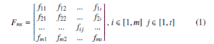
The traffic flow data is time series data, and the change patterns of the traffic flow of adjacent roads in the spatial position have high similarity, which implies the common characteristics of the traffic flow changes. In order to extract this specific feature, we can construct the historical traffic data on all relevant roads into a matrix form, As shown in the following formula, suppose there are related roads in total, and the time series length is t, and f_ij represents the traffic value of the road number i at time j.

The NMF algorithm is used to analyze and decompose matrix data. Its definition is that for any given two-dimensional nonnegative matrix, it can be decomposed into two non-negative submatrices to satisfy the multiplication of these two non-negative matrices to get the original matrix. As shown in (2).

Among them, W is called the basis matrix, and H is called the coefficient matrix or the characteristic matrix. In paper, the H matrix is used as the feature matrix of the original data to achieve the goal of dimensionality reduction and feature extraction. Since both W and H matrices are unknown, they need to be solved by algorithms. Although there are many ways to reduce the matrix dimension, we need to ensure that the values in W and H are non-negative, because all traffic flow values need to be non-negative.

Therefore, the NMF(F, k) algorithm is used to solve the characteristic matrix. At this time, the problem becomes that, given the original non-negative matrix and parameters, matrix factorization can be formulated as a non-negative factorization minimization problem[14]. As shown in the (3):

The NMF(F, k) algorithm first needs to define a cost function to quantify the degree of approximation between F and WH. One way is to use the square of the Euclidean distance between F and WH, as follows:

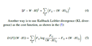
Since this paper needs to use the NMF algorithm to extract the flow characteristics of the relevant roads, it pays more attention to the distribution characteristics of the flow instead of the absolute difference in the flow value. And the KL divergence is often used to measure the similarity of the two distributions. Therefore, the KL divergence is selected as the cost function, and the problem of solving W and H is transformed into: Under the constraint condition W, H ≥ 0, with W and H as parameters, minimize the cost function D(F||WH).

Use the multiplication update rule to iteratively update the parameters W and H. The update equation is as shown in the (6):

In the above update rule, when W and H are at the stagnation point of the divergence formula, the divergence will no longer be updated. The proof of the convergence of the above update equation is given in [14]. Based on the NMF(F, k) algorithm, the basic matrix W and the corresponding feature matrix H are obtained. In the NMF-AttLSTM model, we mainly input H as a feature into the AttLSTM model to provide upstream and downstream spatial features for traffic flow prediction.

2.2        Construction of Attention-LSTM Model

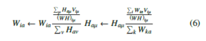
LSTM is a recurrent neural network, as shown in Figure 1. RNN is usually used to deal with time series problems. RNN uses a series of historical data as input, extracts features through non-linear functions, and stores the features extracted from each layer to provide feature information for subsequent calculations. Circulation makes information continue to pass to the next layer.

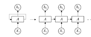
Figure 1: Recurrent neural network (RNN)

However, compared with the conventional RNN, the structure of this repeated module A of LSTM is more complicated, as shown in Figure 2.

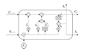
Figure 2: The structure of LSTM cell

This module consists of three parts, the forgotten gate, the input gate and the output gate. σ is the Sigmoid function, output a value between 0 and 1, describing how much of each part can pass.

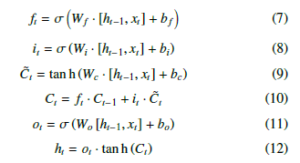
Among them, f_t determines how much information we want to discard. i_t determines how much new information we should add. o_t determines how much information we want to output. x_t is the input at time t. h_t−1 is the output of the previous gate, W_f , W_i, W_c and W_o is the weight, b_i, b_f , b_c and b_o is the bias, C_t−1 is the cell state at the previous moment, C_t is the cell state at the current moment. Since the model is difficult to learn information at a time far from the current time, and it may be important for the current value. To overcome the weakness, we tried to add an attention layer to the LSTM network. Referring to the attention implementation steps of[10], we can apply it to the LSTM model. As shown in Figure 3, the attention layer is added to the LSTM model.

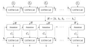
Figure 3: The process of adding an attention layer to the LSTM model

Among them, X_i,i ∈ (1,n) is the input, h_i is the intermediate output result of each cell, all of h_i are input into each attention model as H, and the elements of the next layer h_i are used as H_i to calculate the similarity and weight coefficient, and finally get the attention coefficient. The specific attention model is shown in Figure 4.

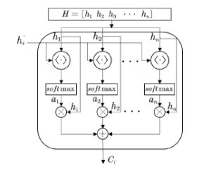Figure 4: The internal structure of attention model

where h·i represents the dot product operation, which is used to calculate the similarity between the current element and the intermediate output result in the previous layer, and then normalized by the softmax function to obtain the corresponding weight coefficient a_i. Finally, a weighted summation operation is performed to obtain the Attention value C_i. The equations used in the attention layer are as follows:

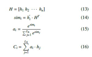
In (14), it uses vector and to calculate similarity to obtain weights, (15) uses the softmax function to normalize the weight, (16) uses the normalized weight a_i and h_i weighted sum. The result of weighted summation is the attention weight value C_i. The implementation of the Attention layer is to retain the intermediate output results of the input sequence by the LSTM encoder, and then calculate the similarity between the intermediate output results of the previous layer and the current output to obtain the weight factor, and finally obtain the attention coefficient. Through the Attention mechanism, it is possible to find out the traffic flow in the past period that is most relevant to the forecast period in the time-based long traffic flow sequence, which improves the ability of the original model to predict a longer sequence traffic flow.

2.3        NMF-AttLSTM

In general, the traffic flow of a road is not only related to its own historical flow, but the flow of its upstream and downstream roads in space also has an important impact on the changes in its own flow. Full consideration of the flow changes in the upstream and downstream roads is of great significance to the current road flow prediction. The definition of the upstream and downstream roads in the spatial position of a road is as follows: based on the direction of vehicle movement, all roads connected to the entrance of the road are called upstream roads, and all roads connected to the exit of the road are called downstream roads, As shown in Figure 5.

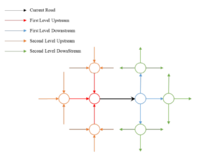
Figure 5: Schematic diagram of the first and second level upstream and downstream roads

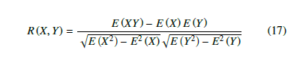
As shown in Figure 5, we consider the first and second level upstream and downstream flow data of the current road. However, in the first and second level upstream and downstream roads, it cannot be guaranteed that all the road traffic has a high correlation with the current road flow. The similarity calculation method is used to calculate the similarity of the flow of all relevant roads with the current road, and the roads with weaker correlation are eliminated accordingly. The addition of the flow characteristics of these roads is not conducive to the improvement of the prediction accuracy. This paper proposes to use the weekly average Pearson correlation coefficient to measure the similarity of the flow changes between the current road and the related road. The Pearson correlation coefficient is generally used to analyze the similarity between two ordered vectors of equal length. The equation is as shown in (17):

Where E is the mathematical expectation. As the traffic flow changes have a certain periodicity, for example, the weekly traffic changes of a certain road section are similar, as shown in Figure 6:

It shows that a week’s traffic flow change can represent the overall traffic flow change of the road section, and the average of the Pearson correlation coefficient of the flow data of a week can be used as the similarity value between the road section and other road sections.

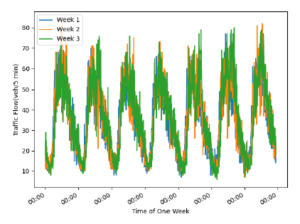
Figure 6: Traffic flows in link 10483 of Wuhan for three weeks

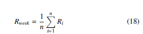
Then the weekly average correlation coefficient can be expressed as the equation (18), n is the number of days, the value is set to 7, and R_i is the day correlation coefficient. Figure 7 is a flowchart of the overall architecture of NMF-AttLSTM.

3. Experimental and Analysis

3.1        Data Sources

• PeMS public data set

The Caltrans Performance Measurement System (PeMS) is a professional traffic flow data collection system. Approximately 15,000 detectors located in major cities in California collect traffic data every day. This paper uses a total of 32 relevant road traffic data from January to March 2017. The traffic data set is counted as 5 minutes, which means that there will be 12 traffic data points per hour. For some missing and abnormal data, the method of moving average is used to fill and correct the abnormal value. In order to obtain the similarity between each road section, a week of data was selected to calculate the weekly average Pearson correlation coefficient, the remaining data was divided into training set and test set, and the effectiveness of the model was evaluated on the test set.

• Wuhan City Traffic Data

To verify the prediction effect of the model on the actual road section, the road section 14394 in the core area of Wuhan was selected as the research section, and a total of 30 related road sections in the upstream and downstream were extracted. The relationship between the upstream and downstream is shown in Table 1.Including road traffic data from November to December 2020. The data collection granularity is 5 minutes, which means that 288 data will be collected for each road section every day. Same as the PeMS data set, the abnormal and missing data are also corrected accordingly. And use one week of data to calculate the weekly spatial correlation coefficient, to select high-correlation road sections to extract spatial features. The actual spatial relationship between section 14394 and its upstream and downstream sections is displayed in QGIS[15] by using OpenStreetMap, as shown in Figure 8.

Table 1: Link number 14394 corresponds to the link number of the upstream and downstream sections

Current Road	Upstream link	Downstream link
14394	14310,14318,14319, 14322,14388,14390, 14392,14393 ,14395, 14397,14398,14742, 14743,32433,32434, 14400,14405	14199,14197,14198, 14200,14313,14317, 14314,14315,14316, 14222,14223,14195, 32344

3.2        Experimental Setup

A sliding time window is used to construct a data set of historical data of this road section and its related road sections. The specific process is shown in Figure 9, where S _t represents the characteristic matrix of historical time series data. Assuming that the input sequence length is 10, the prediction lag time is 15 minutes. Since the data is at a granularity of 5 minutes, it moves backward two time units in turn to extract the current road flow as the label. Now the data set is row₁ : (x₁ : s₁ s₁₀, f₁ : s₁₃), row₂ : (x₂ : s₂ s₁₁, f₂ : s₁₄),…. By analogy, other data set with different input sequence lengths are constructed.

Due to the many parameters of the proposed prediction framework model, the prediction results are also affected. The important parameters are shown in Table 2. Through related experiments, the most suitable parameters are selected as the benchmark parameters for the experiment.

The model in Figure 9 is used for comparative analysis with the NMF-AttLSTM model.

• SVR[16]: Support Vector Regression (SVR) is a method that uses support vector machines (SVM) to solve regression problems, and is often used for time series forecasting. And use RBF as the kernel function.
• LSTM[6]: Which has good predictive ability for time series problems.
• AE-LSTM[8]: Use AutoEncoder to obtain the characteristics of the upstream and downstream traffic flow data of the internal relationship of the traffic flow, and then use the acquired feature data and historical data to predict through the LSTM network.
• AttLSTM[1]: Use the attention mechanism to extract features, add a layer of AttentionDecoder to the LSTM network, so that the model can extract more valuable information.

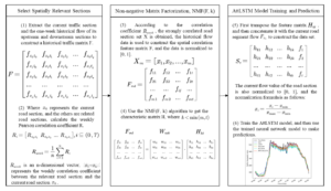
Figure 7: The flow chart of the traffic flow prediction architecture of the NMF-AttLSTM method. The entire prediction process is divided into selection of spatially relevant sections, Non-negative Matrix Factorization (NMF) and AttLSTM model training and prediction. The upstream and downstream sections selected through correlation analysis are used as the input of NMF(F, k), and the feature matrix after dimensionality reduction of the NMF algorithm is spliced with the current section flow as input topredict future traffic flow

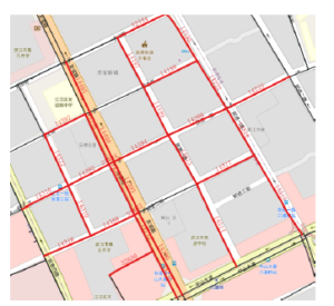
Figure 8: Link 14394 and its upstream and downstream sections in Wuhan urban area

As shown in Table 2, we selected about 30 upstream and downstream road sections related to the current road section, and then based on related experiments, determined that the road section with a circumferential spatial correlation coefficient greater than 0.5 would be selected, and the data is reduced by the NMF algorithm.

The size of the parameter k in the NMF algorithm is equal to the dimension of the feature matrix after dimensionality reduction. For the proposed model and the contrasted neural network model, the hyperparameters are set to the same value. The learning rate is 0.001, the optimization algorithm chooses the adam algorithm, and the mean square error (MSE) is used as the loss function.

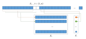
Figure 9: Constructing a data set through a sliding window

3.3        Model Evaluation

In the experiment, the performance of the traffic flow prediction model is measured by three indicators: Mean Absolute Percentage Error (MAPE), Root Mean Square Error (RMSE) and Mean Absolute Error (MAE).

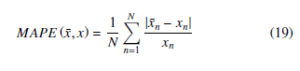
Table 2: Parameters set by default in the experiment

Parameter	Description	Value
n	Number of relevant sections of upstream and downstream	30
Rweek	Weekly average Pearson correlation coefficient	>0.5
τ	Input time series data length	12,24,36
λ	Learning rate	0.001
	Batch Size	16
	Hidden layer neuron	64
	Prediction interval	15min

x¯_n represents the predicted value, x_n represents the observed value, and N represents the number of data. MAPE considers the closeness of the true value to the predicted value and the ratio of the error to the true value, which is often used as a measure of the accuracy of the prediction in the prediction problem. RMSE is used to measure forecast stability. MAE is used to evaluate how close the predicted results are to the real data. The smaller the value, the better the fitting effect.

3.4        Experimental Results

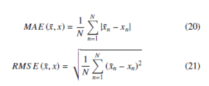
First, use the PeMS public data set for analysis. For different NMF(F, k) algorithm parameters k, under the condition that the input sequence length is 12 and the prediction interval is 15 minutes, the distribution of MAPE is shown in Figure 10. When the parameter k is 5, it has the lowest MAPE error. Here, the parameter k of the NMF algorithm is also equivalent to the reduced dimensionality of the historical data matrix. In subsequent experiments, both the NMF-AttLSTM model and the AE-LSTM model use 5 as the reduced dimension.

We use one day’s data to measure the performance of the NMFAttLSTM model and other comparison models. At the same time, we set three different input sequence data lengths, 12, 24, and 36. They represent the use of 1-hour, 2-hour, and 3-hour historical data as the model input to predict the traffic flow after 15 minutes. Table 3 shows the performance of each model at different input sequence lengths. The results show that as the input sequence length increases, the MAPE, MAE, and RMSE of the AttLSTM model and NMFAttLSTM model decrease, which proves that the model with the attention mechanism is more advantageous than other models when the length of the input sequence increases, because the model with the attention mechanism can extract more important features from the long sequence input. Under the same input sequence length,

the NMF-AttLSTM model and the AE-LSTM model have better performance than other models. Due to the addition of upstream and downstream related road section features, the model provides the characteristics of traffic flow changes. In all the experimental results, the proposed NMF-AttLSTM model has the lowest MAPE, which proves that the model can not only use the spatial characteristics of traffic flow changes, but also obtain more important features from historical flow data, enhancing the prediction ability of neural network model for traffic flow.

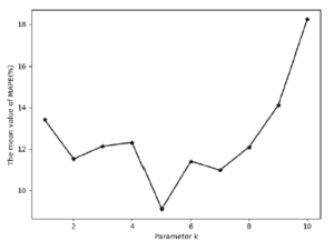
Figure 10: MPAE error of NMF-AttLSTM model under different dimensionality reduction parameter k (PeMS)

Table 3: Performance comparison of models under different input sequence lengths (PeMS)

Input Length	Model	Error Value
		MAPE(%)	MAE	RMSE
12	SVR LSTM AttLSTM	12.43 12.52 10.96	24.00 27.68 26.02	30.96 35.65 34.92
	AE-LSTM	12.15	36.65	46.96
	NMF-AttLSTM	9.10	22.72	31.49
24	SVR LSTM AttLSTM	12.23 13.20 10.50	24.31 25.32 26.30	32.85 31.88 34.57
	AE-LSTM	8.60	22.23	30.41
	NMF-AttLSTM	8.48	21.46	29.27
36	SVR LSTM AttLSTM	12.91 11.53 9.07	29.28 25.84 24.61	37.59 33.45 32.54
	AE-LSTM	9.29	22.45	30.08
	NMF-AttLSTM	7.89	15.21	19.92

In order to verify the effectiveness of the proposed model on the actual road section, the road section 14394 in the core area of Wuhan is selected for analysis. The specific location is shown in Figure 7. According to the method proposed in Section 2.3, firstly, the correlation between each upstream-downstream road section and the current road section is calculated by using the weekly spatial correlation coefficient, Finally, the correlation coefficients of the upstream and downstream sections with a correlation greater than 0.5 with 14394 are obtained, as shown in Table 4. Among the 30 upstream and downstream road sections, 14 relevant road sections are selected. The historical flow data of these 14 relevant road sections are used to construct the historical data matrix F, and then the NMF algorithm is used to obtain the traffic flow spatial characteristics H. For the NMF(F, k) algorithm, the effect of different k on the results was also tested. As shown in Figure 11, the results show that k is 7 with the lowest MAPE.

Table 4: Weekly spatial correlation coefficients of relevant sections in the upstream and downstream of road section 14394 of Wuhan

Upstream	Downstream
Correlation Link ID coefficient	Correlation Link ID coefficient

stream sections are all branch sections, compared with PeMS, the flow value is generally low, so its MAPE error is higher, MAE and RMSE error are lower.

Table 5: Performance comparison of each model (Wuhan)

Model	Error Value
	MAPE(%)	MAE	RMSE
SVR	22.92	3.27	4.39
LSTM	20.40	3.35	4.75
AttLSTM	18.35	3.29	4.75
AE-LSTM	18.75	3.16	4.22
NMF-AttLSTM	16.54	3.01	4.13

Figure 12: The prediction result of each model under the condition that the input

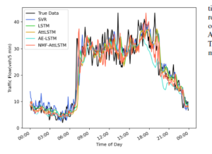
Figure 13: The prediction result of each model under the condition that the input sequence length is 12 (Wuhan)

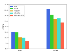
Figure 14: Comparison of MAPE errors of different models in PeMS and wuhan datasets

Table 6 shows the comparison results of the PeMS data set and the wuhan data set. Under the condition that the prediction interval is 15 minutes, the experimental results of the PeMS data set show that the MAPE of the NMF-AttLSTM model is reduced by 1.68% compared with the AttLSTM model and 1.52% compared with the AE-LSTM model. The experimental results of the wuhan data set show that the MAPE of the NMF-AttLSTM model is reduced by 1.81% compared with the AttLSTM model and 2.21% compared with the AE-LSTM model. As shown in Figure 14, NMF-AttLSTM has the lowest MAPE error on both data sets. The results on different experimental data sets prove the effectiveness of the proposed NMF-AttLSTM model.

Figure 12 and Figure 13 respectively describe the results of using one day’s data prediction on the PeMS and Wuhan datasets. It can be seen that the results of the proposed NMF-AttLSTM model fit better with the true values. Figure 15 is the cumulative distribution function (CDF) diagram of the MAE error of the prediction results of each model. CDF can describe the probability distribution of the MAE error. The result shows that the MAE error of NMFAttLSTM on PeMS is less than 20, accounting for more than 60%. The MAE error on the Wuhan dataset is less than 5, accounting for more than 80%, which is better than other models.

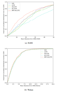
Figure 15: The CDF of MAE error for different models of PeMS and Wuhan data sets

4. Conclusions

The paper studies the method of using the temporal and spatial characteristics of traffic flow to predict traffic flow, and proposes a shortterm traffic flow prediction framework based on the NMF-AttLSTM model. First, analyze the correlation between each upstream and downstream road section and the current research road section by using the weekly spatial correlation coefficient, and eliminate the road sections with low correlation. Then use the NMF algorithm to extract the features of the selected road sections, and finally combine the extracted features with the historical traffic information of the current road section, and use the AttLSTM model for training and prediction. The algorithm considers the spatial relationship of traffic flow, effectively utilizes the flow information of upstream and downstream sections, and also reduces the dimension of data.

In addition, an attention mechanism is added to the LSTM model, so that the LSTM model can extract more valuable features from historical data. This research only considers the relevant flow information of the upstream and downstream sections. In the subsequent work, we can consider adding more complex road network topology information to improve the performance of the model.

5. Acknowledgment

This work is supported by “The wisdom decision-making construction of Wuzhi platform in Wuhan traffic management(ZSHJ-WHSFW-2018-658)”.

1. D. Chen, C. Xiong, M. Zhong, “Improved LSTM Based on Attention Mech- anism for Short-term Traffic Flow Prediction,” in 2020 10th International Conference on Information Science and Technology (ICIST), 71–76, 2020, doi:10.1109/ICIST49303.2020.9202045.
2. B. M. Williams, P. K. Durvasula, D. E. Brown, “Urban Freeway Traffic Flow Prediction: Application of Seasonal Autoregressive Integrated Moving Aver- age and Exponential Smoothing Models,” Transportation Research Record, 1644(1), 132–141, 1998, doi:10.3141/1644-14.
3. Y. Zhang, Y. Xie, “Forecasting of Short-Term Freeway Volume with v-Support Vector Machines,” Transportation Research Record, 2024(1), 92–99, 2007, doi:10.3141/2024-11.
4. M. Duan, “Short-Time Prediction of Traffic Flow Based on PSO Optimized SVM,” in 2018 International Conference on Intelligent Transportation, Big Data and Smart City (ICITBS), 41–45, 2018, doi:10.1109/ICITBS.2018.00018.
5. M. Tan, S. C. Wong, J. Xu, Z. Guan, P. Zhang, “An Aggregation Approach to Short-Term Traffic Flow Prediction,” IEEE Transactions on Intelligent Trans- portation Systems, 10(1), 60–69, 2009, doi:10.1109/TITS.2008.2011693.
6. Z. Zhao, W. Chen, X. Wu, P. C. Y. Chen, J. Liu, “LSTM network: a deep learn- ing approach for short-term traffic forecast,” Iet Intelligent Transport Systems, 11(2), 68–75, 2017.
7. R. Fu, Z. Zhang, L. Li, “Using LSTM and GRU neural network methods for traffic flow prediction,” in 2016 31st Youth Academic Annual Conference of Chinese Association of Automation (YAC), 324–328, IEEE, 2016.
8. W. Wei, H. Wu, H. Ma, “An autoencoder and LSTM-based traffic flow predic- tion method,” Sensors, 19(13), 2946, 2019.
9. D. Bahdanau, K. Cho, Y. Bengio, “Neural machine translation by jointly learn- ing to align and translate,” arXiv preprint arXiv:1409.0473, 2014.
10. A. Vaswani, N. Shazeer, N. Parmar, J. Uszkoreit, L. Jones, A. N. Gomez, L. Kaiser, I. Polosukhin, “Attention is all you need,” arXiv preprint arXiv:1706.03762, 2017.
11. Z. Hao, M. Liu, Z. Wang, W. Zhan, “Human behavior analysis based on attention mechanism and LSTM neural network,” in 2019 IEEE 9th Interna- tional Conference on Electronics Information and Emergency Communication (ICEIEC), 346–349, IEEE, 2019.
12. Z. Wang, J. Poon, S. Sun, S. Poon, “Attention-based multi-instance neural network for medical diagnosis from incomplete and low quality data,” in 2019 International Joint Conference on Neural Networks (IJCNN), 1–8, IEEE, 2019.
13. http://pems.dot.ca.gov/
14. D. Lee, “Algorithms for non-negative matrix factorization,” Advances in Neural Information Processing Systems, 13, 2001.
15. https://www.qgis.org/en/site/
16. H. Drucker, C. Burges, L. Kaufman, A. Smola, V. Vapnik, “Support vector regression machines,” Advances in neural information processing systems, 9(7), 779–784, 2003.

(Click Here)