1. Introduction

Computer vision techniques are usually complex and time consuming, since every pixel of the input image needs to be processed through them. Saliency detection is the technique of finding the salient or important region in an image. So, researches in this field have become popular to reduce this type of computational complexities and shrink the search space of an input image in various vision related applications including object detection, action recognition, image segmentation, video surveillance, medical data processing, robotics and many more. Color contrast present between the salient region and the background is the most popular cue for saliency detection. Another prior that produces good result is the boundary prior which assumes that the boundary regions are mostly backgrounds. These are two popular and successful cues in saliency detection solutions. But, those cues are challenged when the salient regions have less color dissimilarities with the background, they are closer to the border or touch the boundary regions. In those complex conditions, relying only on contrast and boundary priors may not produce good results. So, a different method which does not exclusively rely on contrast based dissimilarities is presented in this study. Experimental results with popular standard datasets and comparison with other state of the art techniques proves the superiority of the proposed system. Evaluation is done based on PR curves and F-Beta measures using publicly available state of the art benchmark results of different studies.

2. Related Works

Since there is usually a visible contrast between the salient region and its background, many researchers mostly relied on contrast prior. Moreover, boundary prior offered promising results in most of the cases.

Early saliency based researches emphasized on center prior which assumes that the salient regions are usually at the center of an image. Those methods usually biased the center of the image with higher saliency values. It was not always true and there are many examples where the saliency is not at the center of an image. So, it was a fragile assumption and nowadays researchers are not much interested in that cue.

On the other hand, boundary prior is an opposite assumption to center prior. Unlike its counterpart, it works better for objects which are not strictly at the center of an image. Although this assumption has some drawbacks, it resulted in better detection in many researches. This prior does not consider the condition where an object contains some of the boundary parts. In [1] the shortest-path distance from an image region to its boundary is used as a cue for saliency detection. It shows that the boundary pixels can easily be connected to the image background instead of the foreground. As a result, it results in incorrect detection if an object is touching the boundary region.

In [2],the authors have taken into consideration the problems of boundary prior and introduced weighted boundary connectivity to successfully solve them and presented a better boundary prior based implementation. They also have proposed a robust optimization technique to combine multiple saliency cues to achieve cleaner saliency maps.

In [3], the authors have used contrast based spatial features along with boundary prior to generate their state of the art saliency detection result. They measured region based color dissimilarity of a superpixelized image found by applying the SLIC algorithm on an input image and suppressed the background using boundary prior as a cue to it. They also have combined the contrast based salient region with boundary based output and fine-tuned the combined saliency map using Gestalt thresholding technique to generate the final salient region.

In [4], the authors have presented a color map based saliency detection technique. It is the weighted average of various color channels. They combined it with border map to acquire the final saliency output. This color map is used successfully in [5] to calculate salient region in an image.

Seam is an optimal 8-connected path of pixels in an image. It is introduced by Avidan et al. in [6] for content aware image resizing and suggested for image enhancement too. Yijun et al. has used seam information in their saliency detection technique [7] with success.

Many methods including [8]–[12] have combined multiple saliency maps to produce better optimized versions successfully. Some of them became complex and their implementation and performance in real world situations are still to be tested. In [13], saliency detection problem has been solved using graph based manifold ranking. In [14], a color and spatial contrast based saliency model is presented which uses four corners of an image to detect the image background. That method was inspired by reverse-management methods and it also applied energy function to further optimize foreground and background.

In [15], a regional contrast based saliency detection method is presented. They show that there are local and global contrast based saliency detection methods. Local contrast based methods commonly produce higher saliency values near object edges and fail to highlight the entire salient region. On the other hand, they criticized some global contrast based methods for being insufficient to analyse common variations in natural images. Inspired from biological vision they propose a histogram-based contrast method and a region based contrast method including spatial information for saliency detection.

In [16], the authors have proposed a saliency detection approach based on maximum symmetric surrounds. They used the low level features of luminance and color. They narrow down the search area for symmetric surrounds as they approach the borders. The disadvantage of their method is that if the salient region touches the border or is cut by the border, it cannot detect it and is treated as the background.

So, there are biologically inspired methods and computationally optimized methods, local and global contrast based methods. There are also combinations of biological and computational models. In [17], a biology based method is used in [18] to extract the feature map and they used graph based approach to normalize the output. Some of the methods computed the entire feature map or some combined multiple maps to produce the final saliency model.

According to the previous discussion, it is obvious that the main challenges of saliency detection problem are low color dissimilarity of objects with its surrounding regions, size and position of a salient region in an image, computational complexity and usability of the method in real life applications. In this study, a combination of seam and color map based salient region detection technique is presented. The proposed method is easy to implement and does better than the other compared methods in response to the mentioned challenges. Details of the proposed method are presented in the following section.

3. Proposed Method

In this study, a novel approach is presented that combines seam and color map based saliency detection procedures in addition to traditional contrast and boundary prior based methods. Moreover, introduction of the quadratic equation based optimization method has improved the result significantly.

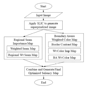
Figure 1: Flow chart of the proposed method.

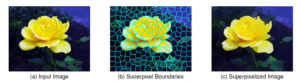
Figure 2: The SLIC approach to transform the input image into superpixels.

Structure of the proposed method is shown in the flowchart of Figure 1. The raw input image is transformed into superpixel image. Seam and color importance maps are generated from this superpixelized image. These two saliency maps are then combined and optimized using a suitable optimization procedure to generate the final saliency map. There are more internal steps seen in the flow chart. In this section the components of this flowchart are discussed in details.

3.1    Superpixel Image

At first, the input image is converted into superpixels using the SLIC method [19]. It groups similar pixels together using some clustering methods around randomly chosen pixel centers. Each region contains the averaged pixel intensity value in that region. It is done to speed up the calculation procedure. Since, working in pixel level will require more time to complete the calculation, it assigns a region ID to each pixel and computation can be continued using those regions only. By doing that the calculation becomes faster and quality is not much considered. It can be converted into the full size image anytime. Our main goal is to detect the salient region only. So, pixel level perfection is not necessary. Figure 2 depicts how an input image is transformed into its superpixel form. Figure 2(b) shows the cluster boundaries which are generated from Figure 2(a). The final superpixelized image will look like the region base image of Figure 2(c).

3.2    Seam Importance Map

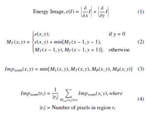
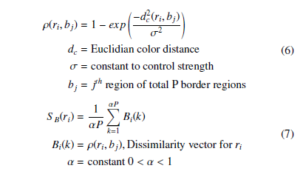
Seam map is computed from the energy map of a given image. It is the cumulative sum of minimum energy values from all four directions of an image namely top to bottom, left to right, bottom to top and right to left. Unlike [6] which computed a seam for the whole image, we follow [7] to get the seam for each pixel of the superpixelized image. The energy function is defined by Sobel operator to get the gradient image using eq. 1 which minimizes the cost. Here, the seam is an optimal 8-connected path of pixels. The superpixelized input image taken as the input to the seam map generation process following [5]. It produces better results as compared to [8] which uses the raw input image in the seam map generation procedure. The reason for this enhancement is the smoothness and stronger edges of the superpixelized image. The computation process is as follows: to compute the seam in the direction of top to bottom, each pixel follows eq. 2. The minimum cumulative sum of energy values of its previous row’s 8-connected neighbours are summed up with the current pixel’s energy value according to eq. 2 to calculate the current pixel’s seam value. Other seam maps are generated in a similar fashion. Since, the background pixels take lower values in any of the four maps as seen in Figure 3, the minimum seam value at each pixel is taken in eq. 3 which suppresses the background well. This way the combined map is found by selecting the minimum of four values for each pixel by eq. 3. The seam map generation process of this study is presented in Figure 3 which shows that Figure 3(b), 3(c), 3(d) and 3(e) are computed from the energy image 3(a); and 3(f) is the combination of seams from Figs. 3(b), 3(c), 3(d) and 3(e). It removes the disadvantage of boundary prior and successfully enumerates the salient object even if it cuts the boundary of an image. The region level seam map is found by averaging seam values in each region as seen in eq. 4. The final seam map is generated by further down-weighting distant regions using average spatial distance as in eq. 5. Pictorial representation of the seam map generation process is visually presented in Figure 3. In this study this seam importance map is combined and further optimized intelligently to produce the final saliency model which does better in conditions where the salient region cuts the boundary.

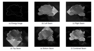
Figure 3: Various stages of seam map calculation method.

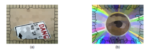
Figure 4: Example of simple and complex border regions.

3.3    Border Contrast Map

Boundary prior is a very successful cue in case of saliency detection. Many researchers have found this cue useful in generating state of the art results. It mainly assumes that boundary regions are mostly backgrounds. This can be easily understood by examining the simple examples and their surroundings in Figure 4. In that figure, the backgrounds of both 4(a) and 4(b) have similar colors like the border regions. Although, Figure 4(a) is simple and have a background similar to the border regions and Figure 4(b)’s boundary regions have several color intensities but all of them constructs the boundary and significantly differ from the salient object or region. To get advantage of this simple but significant characteristic of a digital image, every region is compared with the border regions to find the dissimilarity of that region with the image boundary. In eq. 6 these contrast dissimilarities are computed and the border contrast map is found by averaging the dissimilarities of each region with all boundary regions using eq. 7.

3.4    Color Importance Map

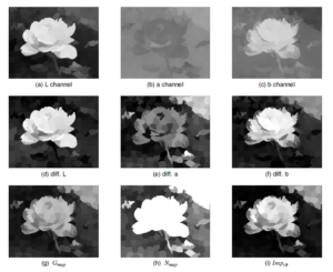
Figure 5: Various stages of computing color map.

A color map in this study consists of the weighted average of different color channels in CIE Lab color space. In a digital image most of the image pixels are backgrounds. So, the main idea of color importance map is to suppress those background pixels by applying some weighting techniques so that the salient regions become prominent. The device independent Lab color space is used to calculate the weighted color map. Because, it provides us more information than RGB color space where all three channels contain similar information. The average L, a and b channels are calculated using eq. 8 and the color difference images are found by subtracting each channel’s average from color intensity values of each pixel as of eq. 9. The visual model of different Lab channels are given in Figure 5. In that figure, the color difference images of Figure 5(d), 5(e) and 5(f) shows remarkable contrasts than its corresponding raw channel images of Figures 5(a), 5(b) and 5(c). The average calculation of the L channel is a bit different. Because, in this channel the intensity values can differ in a range of 0 to 255. Thus the mean and mode can have a large difference and because of frequency, the mode may become insignificant. For this reason, the minimum of (L_mean + L_mode)/2 and L_mean is taken as the weighted average in eq. 8. The Grey map (G_map) in eq. 10 sums up all three channels and Normalized map (N_map) in eq. 11 produces the magnitude value of the color space. These two maps are combined into a single saliency map using eq. 12. Though, gamma correction improves the result very slightly, it is performed on the grey map before the combination in eq. 12 as seen in Figure 5(i). The pixel level color map is transformed into a region level map using the region average in eq. 13. The combined map highlights the salient region significantly, but it also fails at image boundary. So, the border contrast map is introduced with weighted color map in eq. 15 to produce the boundary aware color importance map. 6 shows the boundary aware version of the color importance map. As seen in this figure, the boundary aware color map of Figure 6(c) is found by merging border contrast map of Figure 6(a) and seam map of Figure 6(b). The resulting combination is a better candidate for saliency detection.

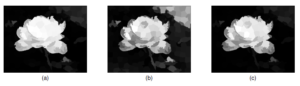
Figure 6: Boundary aware color importance map.

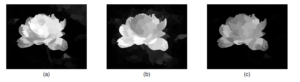
Figure 7: Combination of boundary aware color map and seam map.

3.5     Combining Seam and Color Importance Maps

Following the traditional way of combining saliency maps, the boundary aware color importance map is combined with seam importance map by eq. 16 using multiplication as seen in Figure 7. The combined saliency map of Figure 7(c) is found by merging boundary aware color map of Figure 7(a) and seam map of Figure 7(b). The samples in Figure 7(a) and Figure 7(b) both contain highlighted portions of backgrounds. Though the combined result in Figure 7(c) successfully suppresses the background, it does not enumerate the salient result sufficiently. So, an optimization procedure is required to do the rest of the job.

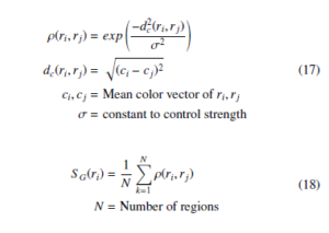
3.6     Color Distance and Contrast Dissimilarity

The existing color contrast between the regions in an image is one of the main attractions of saliency detection studies. The euclidean color distance in the Lab color space of the superpixels is used to measure the contrast difference between the superpixels as in eq. 17. The global contrast map is found by using eq. 18. This is used in the optimization equation as the smoothness weight.

3.7    Optimization

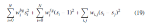
Most of the previous researchers use multiplication or weighted summation to combine multiple saliency cues. The resulting combination does not do well in case of generalization. The main objective of saliency detection techniques is to generate a map closer to the binary ground truth image. So, some authors developed an optimization technique towards this goal. In this research, optimization is done by minimizing their quadratic cost function 19 proposed in [2]. All three terms of this cost function are square errors and it can be solved by using least square method. The first term of the cost function represents the background which forces a superpixel p_i with greater background weight w^bg_i to take a small value s_i closer to

1. In this research, the background weight w^bg_i is 1 − Saliency. The second term represents the foreground which forces a superpixel p_i with greater foreground weight w_i^fg to take a value closer to 1. Here, the foreground weight is one of the saliency maps found in this study. The third term is the smoothness term which smooths both the background and foreground by removing small noises. The color dissimilarity based global contrast map from eq. 18 is used as the weight for the smoothness term. Since the target of this weight is to smooth the combined saliency map, connecting two levels of nearest neighbours and the boundary regions before dissimilarity measures produces better results. In this study, different combinations of saliency measures are used as the foreground and background weight in eq. 19 as shown in table 2 and a balanced combination is proposed as the optimal combination. The optimal saliency map of Figure 8(c) is found by solving the quadratic equation proposed in [2] using 8(a) as background map and 8(b) as foreground map.

4. Experiments and Results

4.1    Datasets

Standard datasets like MSRA 1k, MSRA 10k, CSSD and ECSSD are used to evaluate the performance of this study. Here, MSRA 1k and 10k are subsets of widely used MSRA original dataset which contains 20,000 images along with their hand labelled rectangular ground truth images which are manually annotated by 3-9 users. In [20] and [21], the authors has claimed that the original MSRA dataset has limitations in fine grained evaluation because of being too coarse in some cases. In [21] the authors presented the MSRA 1k or ASD dataset by manually segmenting each salient region which overcomes the limitations of the original MSRA dataset. An extended version of MSRA 1k dataset which contains pixel level binary ground truth images of 10,000 images from the original MSRA dataset is presented in [15]. They named this dataset MSRA10k which was previously called THUS10000. The first row of Figure 9 shows some bounding box annotation from original MSRA dataset and the second row shows the pixel level ground truth annotation from MSRA10k dataset. Almost all modern saliency detection techniques use this dataset as a benchmark for evaluation of saliency detection methods.

MSRA based datasets are good for saliency detection evaluation and contain a large variety in contents, but their backgrounds are relatively simple and smooth. To evaluate the complex situations in saliency detection, where objects and backgrounds have relatively low contrast and object surroundings are comparatively complex, in [12] the authors have proposed CSSD dataset with pixel level binary ground truths in 2013 which is a more challenging dataset with 200 images containing complex situations and they extended the dataset by increasing the images to 1,000 in [22] and named it Extended Complex Scene Saliency Dataset (ECSSD). Some members of CSSD and ECSSD datasets with complex backgrounds and low contrast surroundings are presented in Figure 10.

Table 1: Datasets and compared methods.

Dataset	Compared Methods
MSRA 1k	CA[23], FT[24], HC[15], LC[25], MSS[16], GS[1], SF[10], SWD[26], BARC[3], BARCS[8], BACS[5]
MSRA 10k	GS[1], SF[10], BARC[3], BARCS[8], BACS[5]
CSSD	GS[1], SF[10], BARC[3], BARCS[8], BACS[5]
ECSSD	GR[27], IT[17], SR[28], MSS[16], GS[1], SF[10], BARC[3], BARCS[8], BACS[5]

4.2    Evaluation Metrics

There are usually two types of evaluation strategies for every computer vision technique – qualitative analysis and quantitative analysis. Results found in this study are compared with several state of the art methods which are labelled as HC[15], MSS[16], GB[18], SWD[26], RC[29], AC[30], IT[17], GR[27], LC[25], FT[24], CA[23], AIM[31], GS[1], SF[10], SR[28], BARC[3], BARCS[8] and BACS[5]. Most of these labels are used in previous researches like [21], [15] and [32]. Other labels are constructed by taking some meaningful letters from the titles of the related publications.

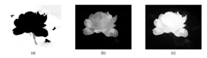
Figure 8: Combination of foreground and background maps to generate the optimal saliency model.

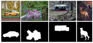
Figure 9: Rectangular annotation of original MSRA dataset and the pixel level ground truth annotation from MSRA10k dataset.

Based on publicly available results for specific dataset, the proposed method has been compared with other state of the art methods as shown in Table 1.

Qualitative analysis of this study are presented in Figure 15 and 16 with some of the mentioned methods containing comparative samples from respective technologies. For quantitative analysis precision recall curves are shown for different datasets along with other techniques that clearly proves the superiority of the proposed method. To draw this precision recall curve simple binarization is performed by varying the threshold in the range from 0 to 255 and the curves are plotted according to the ground truth data available for each input image in the corresponding dataset. Since the only consideration of precision-recall curve is whether the foreground region saliency is higher than the background saliency, to evaluate the overall performance F-beta measures in Figure 14 are also presented in this study to better understand the performance of the compared methods.

4.3    Experimental Setup

Standard datasets are used to evaluate the proposed method. An initial 600 pixel region size is considered for converting the input image into the superpixelized version using the SLIC method. Other static variables are considered as α = 0.25 and compactness = 20.

4.4    Optimization Experiments

Some promising combinations of saliency maps are explored in this study which are briefly discussed in this section. In the proposed optimization method, if the border contrast map is used as the background weight and the seam importance map is used as the foreground weight, we find closer PR curves as seen in Figure 12. The f-beta score is also closer to the proposed method as depicted in that figure. Similarly, different combinations are experimented for this study. Some of them are presented in table 2 and their qualitative and quantitative results are shown in Figure 11 and Figure 12 respectively. The runtime for these three combinations are given in table 3. In all three combinations, the smoothness weight is kept the same which is the global contrast map between the superpixels from eq. 18.

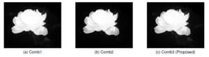
Figure 11: Optimization combinations.

From the results in Figure 11, 12 and runtimes in table 3 it is seen that all three compared methods are closer to each other. But the second combination is the slowest since it introduces more computational complexities and the first combination is the fastest in terms of runtime comparison. On the other hand, for the MSRA 1k dataset the second combination does well in case of PR curve and F-beta test. But, the third one does well in complex situations like the ECSSD dataset. Its performance is also competitive in MSRA 1k dataset and the runtime is quite acceptable in comparison to the fastest method and its excellent performance on the complex dataset. Thus the third combination is chosen as the proposed method in this study and it will be termed as Our method onwards.

Table 2: Proposed optimization combinations.

Method

Foreground

Background

Comb1	Border Contrast Map from eq. 7	Seam Map from eq. 4
Comb2	Border Contrast Map from eq. 7	Combined Seam and Boundary Aware Color Map from eq. 16
Comb3 (Proposed)	Boundary Aware Color Map from eq. 15	Weighted Seam Map from eq. 5

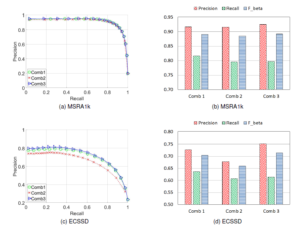
Figure 12: Precision recall curves for different combinations.

Table 3: Runtime comparison of proposed combinations.

Method	Comb1	Comb2	Comb3 (Proposed)
Time (sec)	1.63	2.65	1.745
Code	Matlab	Matlab	Matlab

4.5    Results

The qualitative analysis in Figure 15 and 16 visually demonstrates the performance of the presented method compared to other state of the art techniques. The first row shows the input images and the last row contains the target pixel level ground truths for corresponding input images. From those figures it is seen that the proposed method done quite well with respect to other compared techniques.

In case of quantitative comparison, the precision-recall curve in Figure 13 clearly demonstrates the superiority of the proposed method. As pointed in [15], all methods have the same precision and recall values at maximum recall for threshold = 0 and all pixels are considered to be in the foreground. On the other hand, if the curves are observed from recall value 0.5 to 1, it is realized that for all datasets the proposed method exhibits higher precision values due to smoother saliency containing more pixels in the salient region with saliency value 255 until it reaches to the common minimum precision value at recall = 1 and distinctly remains at the top of other curves until that. When a PR curve shows higher precision values for higher recalls, that is considered better. So, for the given datasets the proposed method clearly outperforms all other methods in terms of PR curve analysis.

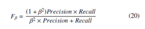
To measure the overall quantitative performance F_β measures are also calculated. In doing so, β = 0.25 is considered in eq. 20 like [8] and [3] to draw F-beta measures in Figure 14. The bars in this figure demonstrate that the presented method clearly surpasses other state of the art techniques.

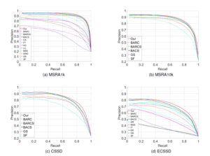
Figure 13: Precision recall curves for different datasets.

The average runtime of different methods are given in table 4 as presented in [15]. The given times are dependent on the programming platform and different machine specifications. It may vary on other computer or programming platforms. So, this is mentioned here only for references. The average runtime of the proposed method is also mentioned in that table. The configuration of the windows machine for this study is a second generation Intel core i5 CPU with 8 Gb of DDR3 RAM.

Table 4: Time comparison of different methods.

Method	Our	AIM	CA	CB	FT	GB
Time (s)	1.745	4.288	53.1	5.568	0.102	1.614
Code	Matlab	Matlab	Matlab	M&C	C++	Matlab
Method	HC	IT	LC	MSS	RC	SWD
Time (s)	0.019	0.611	0.018	0.106	0.254	0.100
Code	C++	Matlab	C++	Matlab	C++	Matlab

5. Conclusion

A novel method of saliency detection is presented in this paper that combines seam and color map based saliency detection procedures. The background and foreground weights proposed for the quadratic eq. 19 have successfully outperformed other state of the art methods and those have never been explored before. Some intermediate combinations are also presented with their detailed comparison. Though, one of the combinations is marked as the proposed solution balancing the runtime and performance, any of them can be used with respect to the application demand. Moreover, the presented results in the experimental section of this study clearly demonstrates the superiority of the proposed method over other state of the art techniques in terms of qualitative and quantitative analysis. The use of standard benchmark datasets strengthens the acceptability of this study and its publicly available results make an opportunity for other researchers to compare their findings with the proposed method.

Computational devices are improving day by day. So, in future exactness of saliency detection technique will be the main concern. Moreover, a fine tuned version of the proposed method is possible and its implementation in an application level programming language like C++ would certainly improve its runtime. Besides that, different saliency weight calculation procedures of this study like border contrast map, color map and contrast based dissimilarity can be parallelized and this way runtime can come to its minimum. So, the future plan is to improve the saliency detection technique performance and apply it into various computer vision related applications like pedestrian detection, action recognition, object detection and recognition etc. Experimenting the proposed model with more complex datasets can be another interesting scope of study.

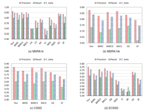
Figure 14: F-beta curves for different datasets.

6. Declaration

6.1    Availability of data and materials

The experimental results of this study are available for download at (https://aminulislam.net/#research). The famous MSRA 10k dataset is freely available at (https:// mmcheng.net/msra10k), the CSSD and ECSSD datasets are available at (http://www.cse.cuhk.edu.hk/_˜leojia/projects/ hsaliency/dataset.html). Other datasets used and/or analyzed during this study are available from the authors upon reasonable request.

6.2    Competing interests

The authors declare that they have no competing interests.

6.3    Authors’ contributions

AI executed the experiments, analyzed results, and wrote the initial draft of the manuscript. SMMA contributed to the concept, edited the manuscript, supervised the project and provided technical support and conceptual advice. The authors reviewed and approved the final manuscript.

6.4    Acknowledgements

We thank all the people who gave us various perceptive and constructive comments.

1. Y. Wei, F. Wen, W. Zhu, J. Sun, “Geodesic Saliency Using Background Priors,” in 12th European Conf. on Computer Vision (ECCV), Proc., Part III, volume 7574, 29–42, Springer, 2012, doi:10.1007/978-3-642-33712-3\ 3.
2. W. Zhu, S. Liang, Y. Wei, J. Sun, “Saliency Optimization from Robust Background Detection,” in Proc. IEEE Conf. Computer Vision and Pattern Recognition, 2814–2821, 2014, doi:10.1109/CVPR.2014.360.
3. S. M. M. Ahsan, J. K. Tan, H. Kim, S. Ishikawa, “Boundary Aware Regional Contrast Based Visual Saliency Detection,” in The Twenty-First Int. Symposium on Artificial Life and Robotics, 258–262, 2016.
4. T. G. Joy, M. M. Hossan, “A Study on Salient Region Detection using Bounday and Color Cue,” Khulna University of Engineering & Thechnology, 2018,
   thesis no. CSER-18-26.
5. A. Islam, S. M. M. Ahsan, J. K. Tan, “Saliency Detection using the Combination of Boundary Aware Color-map and Seam-map,” in International Conference on Computer, Communication, Chemical, Materials and Electronic Engineering (IC4ME2), 2019.
6. S. Avidan, A. Shamir, “Seam Carving for Content-aware Image Resizing,” ACM Trans. Graph., 26(3), 2007, doi:10.1145/1276377.1276390.
7. Y. Li, K. Fu, L. Zhou, Y. Qiao, J. Yang, “Saliency detection via foreground rendering and background exclusion,” in Proc. IEEE Int. Conf. Image Processing (ICIP), 3263–3267, 2014, doi:10.1109/ICIP.2014.7025660.
8. A. Islam, S. M. M. Ahsan, J. K. Tan, “Saliency Detection using Boundary Aware Regional Contrast Based Seam-map,” in Proc. Int. Conf. Innovation in Engineering and Technology (ICIET), 2018, doi:10.1109/CIET.2018.8660825.
9. T. Liu, J. Sun, N. Zheng, X. Tang, H. Shum, “Learning to Detect A Salient Object,” in Proc. IEEE Conf. Computer Vision and Pattern Recognition, 1–8, 2007, doi:10.1109/CVPR.2007.383047.
10. F. Perazzi, P. Kra¨henbu¨ hl, Y. Pritch, A. Hornung, “Saliency filters: Contrast based filtering for salient region detection,” in Proc. IEEE Conf. Computer Vision and Pattern Recognition, 733–740, 2012, doi:10.1109/CVPR.2012. 6247743.
11. A. Borji, M. Cheng, H. Jiang, J. Li, “Salient Object Detection: A Benchmark,” IEEE Transactions on Image Processing, 24(12), 5706–5722, 2015, doi:10.1109/TIP.2015.2487833.
12. Q. Yan, L. Xu, J. Shi, J. Jia, “Hierarchical Saliency Detection,” in Proc. IEEE Conf. Computer Vision and Pattern Recognition, 1155–1162, 2013, doi:10.1109/CVPR.2013.153.
13. C. Yang, L. Zhang, H. Lu, X. Ruan, M. Yang, “Saliency Detection via Graph-Based Manifold Ranking,” in Proc. IEEE Conf. Computer Vision and Pattern Recognition, 3166–3173, 2013, doi:10.1109/CVPR.2013.407.
14. H. Zhang, C. Xia, “Saliency Detection combining Multi-layer Integration algorithm with background prior and energy function,” arXiv preprint arXiv:1603.01684, 2016.
15. M. Cheng, G. Zhang, N. J. Mitra, X. Huang, S. Hu, “Global contrast based salient region detection,” in Proc. CVPR 2011, 409–416, 2011, doi: 10.1109/CVPR.2011.5995344.
16. R. Achanta, S. Susstrunk, “Saliency detection using maximum symmetric surround,” in Proc. IEEE Int. Conf. Image Processing, 2653–2656, 2010, doi: 10.1109/ICIP.2010.5652636.
17. L. Itti, C. Koch, E. Niebur, “A model of saliency-based visual attention for rapid scene analysis,” IEEE Transactions on Pattern Analysis and Machine Intelligence, 20(11), 1254–1259, 1998, doi:10.1109/34.730558.
18. J. Harel, C. Koch, P. Perona, “Graph-based visual saliency,” in Advances in neural information processing systems, 545–552, 2007.
19. R. Achanta, A. Shaji, K. Smith, A. Lucchi, P. Fua, S. Su¨sstrunk, “SLIC Superpixels Compared to State-of-the-Art Superpixel Methods,” IEEE Transactions on Pattern Analysis and Machine Intelligence, 34(11), 2274–2282, 2012, doi: 10.1109/TPAMI.2012.120.
20. Z. Wang, B. Li, “A two-stage approach to saliency detection in images,” in 2008 IEEE International Conference on Acoustics, Speech and Signal Processing, 965–968, IEEE, 2008.
21. R. Achanta, S. Hemami, F. Estrada, S. Susstrunk, “Frequency-tuned salient region detection,” in Proc. IEEE Conf. Computer Vision and Pattern Recognition, 1597–1604, 2009, doi:10.1109/CVPR.2009.5206596.
22. J. Shi, Q. Yan, L. Xu, J. Jia, “Hierarchical Image Saliency Detection on Extended CSSD,” IEEE Transactions on Pattern Analysis and Machine Intelligence, 38(4), 717–729, 2016, doi:10.1109/TPAMI.2015.2465960.
23. S. Goferman, L. Zelnik-Manor, A. Tal, “Context-Aware Saliency Detection,” IEEE Transactions on Pattern Analysis and Machine Intelligence, 34(10), 1915– 1926, 2012, doi:10.1109/TPAMI.2011.272.
24. R. Achanta, S. Susstrunk, “Saliency detection for content-aware image resizing,” in Proc. 16th IEEE Int. Conf. Image Processing (ICIP), 1005–1008, 2009, doi:10.1109/ICIP.2009.5413815.
25. Y. Zhai, M. Shah, “Visual Attention Detection in Video Sequences Using Spa- tiotemporal Cues,” in Proc. of the 14th ACM Int. Conf. on Multimedia, MM ’06, 815–824, ACM, 2006, doi:10.1145/1180639.1180824.
26. L. Duan, C. Wu, J. Miao, L. Qing, Y. Fu, “Visual saliency detection by spatially weighted dissimilarity,” in Proc. CVPR, 473–480, 2011, doi: 10.1109/CVPR.2011.5995676.
27. C. Yang, L. Zhang, H. Lu, “Graph-regularized saliency detection with convex- hull-based center prior,” IEEE Signal Processing Letters, 20(7), 637–640, 2013.
28. X. Hou, L. Zhang, “Saliency detection: A spectral residual approach,” in 2007 IEEE Conference on computer vision and pattern recognition, 1–8, Ieee, 2007.
29. M. Cheng, N. J. Mitra, X. Huang, P. H. S. Torr, S. Hu, “Global Contrast Based Salient Region Detection,” IEEE Transactions on Pattern Analysis and Machine Intelligence, 37(3), 569–582, 2015, doi:10.1109/TPAMI.2014.2345401.
30. R. Achanta, F. Estrada, P. Wils, S. Susstrunk, “Salient region detection and segmentation,” in International conference on computer vision systems, 66–75, Springer, 2008.
31. N. D. B. Bruce, J. K. Tsotsos, “Saliency, attention, and visual search: An information theoretic approach,” Journal of Vision, 9, 5–5, 2009, doi:10.1167/9.3.5.
32. H. Chen, P. Wang, M. Liu, “From co-saliency detection to object co- segmentation: A unified multi-stage low-rank matrix recovery approach,” in Proc. IEEE Int. Conf. Robotics and Biomimetics (ROBIO), 1602–1607, 2015, doi:10.1109/ROBIO.2015.7419000.

(Click Here)