1.Introduction

Ultrasonic waves are commonly utilized in numerous applications such as nondestructive testing (NDT), object recognition, and medical imaging. They have been used as an inspection tool in different materials [1]. Ultrasonic waves can spot any irregularities contained inside the tested specimens that cannot be identified visually. They can be used in different medical devices such as the application of ultrasound imaging for pregnancy [2]. Ultrasonic inspections are listed as a non-destructive testing method because the procedure implemented does not cause any damage to the tested objects [3]. Pulse-echo mode is the most widely used method for inspection. The key benefit of this approach is that only one side of the tested object should be accessible. This broadens its applicability to accommodate for different applications such as crack detection and surface imaging [4].

Several applications include scanning a specimen’s surface in order to obtain an image that represents the object. However, this process should include a 2D or 3D automated scanner coupled with the ultrasonic devices [5]. Therefore, a reliable control system should be designed and implemented to ensure correct images are obtained. The surface imaging can be used in different industrial applications [6]. It can also find several applications in the oil and gas industry. The integrity of the oil well cement placement can play a vital role in the success of the drilling operations. Ultrasonic imaging methods can be used for inspecting the cement integrity. This ensures a good sealing layer is obtained between the well and the formation [7]. The cement integrity becomes a critical issue when extended wells are to be drilled [8].

Many applications require using coupling a scanner with another measuring device e.g. ultrasonic pulser-receiver to record real-time data. Commercial tools that do this job are available and can be easily purchased. These tools were used by different researchers in their projects [9]. However, the cost of these tools might be very expensive. Furthermore, the recorded data from the commercial devices might be limited to certain parameters such as amplitude-based data. This limit can be bypassed when the experiment is manually designed, and the script codes are prepared by the user. Some researchers used an ultrasonic device that utilizes LabVIEW for data acquisition [10]. However, in that application, the ultrasonic device was fixed and hence no movement was allowed.

To the best of the author’s knowledge, there are not enough published articles that focus mainly on the ultrasonic scanner setup. Most of the articles focus on the application of this method instead. This makes it difficult to replicate these experiments without purchasing expensive equipment and services. In this study, the main focus is on the experimental setup that can produce a two-dimensional image of any surface. This setup utilizes equipment that are of lower cost than the commercial setups used in previous studies. The scanner movement and data acquisition process are ultimately controlled through a custom-written script in MATLAB. A pre-programmed microcontroller is used as an interfacial connection between the scanner and MATLAB. An ultrasonic pulser-receiver device is used as the interface between the transducer and MATLAB. This design might attract researchers who are looking for simple and cost-effective surface imaging methods using ultrasonic waves. All the equipment and control systems are addressed in the text. This article is an extension version for a previously published conference paper [5].

2. Pulse-echo Technique Background

Figure 1a displays the principles of this method. A transmitter is used to send out a pulse wave into the body. When a boundary is reached, e.g. the back wall or a deficit in the material, the wave is reflected back towards the receiver where it is captured and recorded [3]. In general, the pulse-echo mode uses the same ultrasonic transducer for transmitting and receiving the waves, as shown in Figure 1b.

Different types of sound waves propagate in materials, such as longitudinal and shear waves. The latter cannot travel in liquids or gases, unlike the longitudinal waves which can exist in any medium [11]. The speed of sound is not constant but depends on the material it passes through. This speed is roughly 340 meters per second in air, 1500 in water and over 2000 in solids. Acoustic impedance (Z), which describes the resistance of a material to sound waves, depends on the density and speed of sound [3]

where c is the speed of sound in the propagating material, whereas ρ is the density of the material.

Ultrasonic waves follow the same principles of acoustic waves. When a wave hits an interface, part of it will undergo reflection while the other part will undergo refraction [3]. The acoustic impedance can be used to determine the reflection and transmission behaviour taking place at the boundaries of two objects in contact. The intensities of the divided waves depend on the material properties at the boundary. Ultrasonic waves of high frequency cannot propagate in air due to their low acoustic impedance; therefore, a wave passing through a solid material will mostly undergo reflection when encountering an air interface. The reflection coefficient (R) can be obtained using [3]

where Z₁ and Z₂ represent are the acoustic impedance of the materials in contact. Three possibilities might be encountered when solving (2), as follows:

1. Z₂ >> Z₁, e.g. solid-air interface, then R equals to 1 which suggests that all the waves are reflected back towards the receiver;
2. Z₁ = Z₂, e.g. two similar materials in contact, then R equals 0, suggesting that all the waves were transmitted to the other end. This means that no signal is read at the receiver.
3. Z₂ < Z₁, then R would be a negative value; this change in sign suggests a phase shift in the signal [3].

Furthermore, as sound travels through a medium, the intensity of the wave reduces due to attenuation. Attenuation is a result of two mechanisms: scattering and absorption. Wave scattering describes the spreading of sound waves in different directions besides its original path, whereas absorption refers to the losses due to energy conversion within the material, e.g. mechanical energy converts to heat. The frequency profoundly influences the degree of attenuation and the medium it propagates in [3].

3. Methodology

3.1. Materials

The main equipment that are used in this experiment are: an ultrasonic transducer, an ultrasonic pulser-receiver, a microcontroller, a scanner, and a PC with MATLAB software. All of these equipment are briefly discussed in the following text.

Ultrasonic transducer – This device is used to transmit and/or receive acoustic energy. A focused ultrasonic transducer of 10 MHz rating was selected for this experiment. The major benefits of using a high frequency transducer is to improve the accuracy and quality of the output image. Generally, unfocused transducers are not used for scanning purposes as they cannot attain high resolutions without the use of extra lenses [12]. Passive focusing techniques could be utilized to improve the accuracy of these transducers [13].

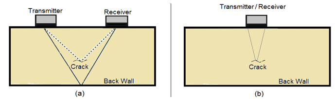Figure 1: Pulse-echo mode. (a) Using two separate transmitter and receiver transducers; (b) Using a single transmitter/receiver transducer (Transceiver)

Ultrasonic waves of high frequencies cannot pass in air. Hence, a connecting fluid is regularly used to provide a medium that allows for wave propagation [14]. Therefore, the ultrasonic transducer was submerged in standing water for the full extent of the experiment.

In order to focus the waves accurately, the exact distance between the transducer and the object to be scanned should be predefined. This will lead to higher resolution for the scanned image. This distance represents the location of the maximum wave intensity and is identified by reading the focal length rating of the transducer. This value will change with different types of transducers.

The focal spot diameter is a critical parameter to be considered during the design stage since it can impact the resolution. If this attribute has a value lower than that of the scanned object, better resolutions would be achieved. The focal spot diameter (d) can be calculated using the following relation [3]:

where d is in mm, l_w and c_w area the speed of sound in m/s and focal length in mm in standing water, f is the nominal frequency in MHz and D is the diameter of the transducer in mm. This relation that exists between the focal spot diameter and frequency is represented in Figure 2 for simplicity. The two parameters are inversely proportional, where a smaller focal spot (better resolution) can be attained using high frequency.

The ultrasonic transducer that was used is displayed in Figure 2 as a red mark. It is of 10 MHz frequency, 25.4 mm element diameter, and 51 mm focal length in water. When using these values in (3), the focal spot diameter can be calculated to be around 0.3 mm in water.

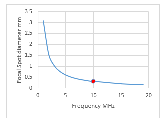Figure 2: Variations of the focal spot diameter with frequency

Ultrasonic pulser receiver (UPR) – This instrument is employed to provide the excitation voltage for the transducer. It can either be manually designed for a given application or purchased from a manufacturing company. The device which was used in this experiment was produced by Lecoeur Electronique. It contains two channels, a transmitter and a receiver. The first channel can be used to direct the electrical pulses to the transducer which then sends out ultrasonic waves. The second channel receives the electrical signals from the ultrasonic transducer when it detects ultrasonic waves. The ultrasonic pulser receiver can be used in two different modes: either in single mode, as a transmitter or receiver, or in full mode, both as a transmitter and as a receiver.

Automated table (Scanner) – This device is used to guide the transducer in different directions. In this experiment, the scanner can move in two horizontal directions. This is the minimum requirements for scanning an area. The movement is employed by the use a dynamic gantry, that is connected onto a lead screw of 250 mm length. The lead screw has a 2mm pitch of 2 mm and four threads (Four Start). Therefore, the regular actual lead of is 8 mm per revolution.

Stepper motors are used to provide rotation for the lead screw and hence, movement of the gantry. The stepper motors utilized have a high torque value of 114 oz. These motors must undergo 200 steps to complete a full revolution. Hence, a 40 mm linear displacement per step can be easily achieved. Two stepper motor drivers (DRV8825) were used to control the motors. Each driver can deliver a maximum of 45 V output voltage and 2.5 A current. The drivers employ two current sinewaves along with a phase shift of 90 ̊. This allows a smoother motor operation. Additionally, the drivers can be used in micro-stepping modes. In this experiment, steps of 100 mm where used.

Figure 3 shows the assembled materials. The automated table was fixed to a larger supporting frame. A clamp, made up of polycarbonate material, was fixed to the lower end of the automated table. This clamp was used to hold the ultrasonic transducer. Limit switches were installed at the ends of the lead screw to prohibit any movement beyond a given limit to avoid stalling of the motor.

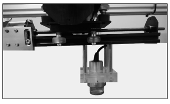Figure 3: Assembly of the experimental setup

A micro-controller electronic board, that is coded using C++ language, was used to provide suitable control over the stepper motors. In addition to that, it allows for micro-stepping to be attained. This board consists of 6 analogue inputs and 14 digital input/output pins. The connection circuit for the scanner is displayed in Figure 4. The micro-controller is connected to a power supply through an adaptor (Not shown in figure) and to the PC through a USB cable. The microcontroller is connected to the stepper motor drivers using the pins. This allows direct control of the drivers which in turn excite the motors when triggered. A transistor is used in this connection to amplify the electronic signal delivered by the power supply to the motor drivers.

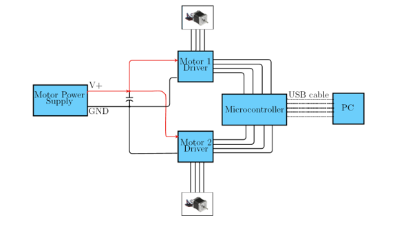Figure 4: A connection circuit for the scanner.

3.2. Control System

The control system can be divided into 3 main categories: The ultrasonic pulser receiver circuit, the automated table circuit, and the overall system circuit. The control mechanism for these categories are briefly discussed in the following text.

Uultrasonic pulser receiver circuit – The UPR device operates with a script developed in MATLAB. The script enables a series of attributes to be modified including the pulsed frequency, exciting voltage, gain, and others.

The excitation voltage of the ultrasonic pulser receiver is limited to a range of 100 V up to 230 V. The transducer rating  can be excited by applying pulsed voltages in from 100 V up to 300 V. This oscillates the inner piezoelectric crystal and produces ultrasonic waves. If the excitation voltage is increased, the reflected signal will record a higher amplitude which can be beneficial when significant wave attenuations are expected.

The gain, which is a signal amplification, is another important parameter that can be regulated to counter the effect of signal attenuation. The recorded signals are not always measurable without tuning the gain value. The ultrasonic pulser receiver is limited to a 80 dB amplification. Nevertheless, laboratory experiments have shown that the measurements become skewed when this is set to 60dB or higher. This is due to increased impact of noise. Therefore, a gain of 40 dB was used in this application.

The pulsed frequency was fixed at 10 MHz to match the ultrasonic transducer rating. The pulsed width can also be controlled. This width is small, but it can be calculated by analyzing both the amplitude and length of the reflected wave. The assigned pulsed width was nearly 4 ms.

The pulsed repetition frequency is also regulated by MATLAB. To identify the minimum pulsed repetition time needed for the oscillation of the transducer, it is necessary to obtain the time for each reading to be obtained. This attribute considers the time for the wave to propagate within various materials or layers. In the present scenario, the waves travel through standing water. The interval distance in water between the coin and transducer should be regulated to maintain the coin I the range of transducer’s focal length.

The total travel time of the wave (TWT) should be estimated to determine the pulsed repetition frequency. This parameter takes into account the wave transmission and reflection time in water. To find TWT, the interval distance between both the transducer and coin should be defined. The following relationship can be used:

where WD is the interval distance / depth of water (51 mm), and c_w is the speed of sound in standing water (1500 m/s). Adding the value of TWT from (4), which equals 68 ms, to the pulse width gives the minimum total pulse time needed. The pulse width is much smaller than the TWT value. Assuming 200 ms was the pulse repetition time chosen to ensure no more reflected and scattered waves will affect the reading, a 5 kHz pulse repetition frequency would be required. This is achievable using the UPR device. However, the scanning speed is mainly affected by the speed of the automated table, which requires 0.1 seconds interval time to process and act to the movement commands (see text below). This suggests that even a very low pulse repetition frequency can work. In this experiment, a pulse repetition frequency of 1 kHz was chosen as it allows for multiple measurements at each location (lower values could have been used).

Automated table circuit – This circuit is controlled by a microcontroller as shown in Figure 4. A serial interface was developed between MATLAB and the microcontroller using a computer that provides full control over the movement of the device via MATLAB. The script allows for two modes of directional movement:

• To an absolute position,
• Specified number of steps in each direction.

The purpose of this experiment is to scan the area and record the data at each location. As a result, it was found that controlling the movement by predefined steps would be more appropriate. The total scanning time should be minimized and therefore, the automatic table was designed to scan in a zigzag mode.

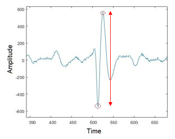Figure 5: Waveform

In general, data points should be closer to one another in order to improve the resolution of the image. This requires setting short intervals between each scanned location. However, this will lead to an increase in the overall scanning time.

 Overall system circuit – MATLAB is employed to provide the main control over the whole system. This approach was achieved by integrating control circuit of the Ultrasonic Pulser-Receiver and scanner. The script has been adapted to obtain three pulses at each position. This is useful in reducing the possible errors during measurement. Figure 5 shows an example of a recorded pulse wave. Figure 6 shows a schematic of the main control process.

The time duration between scanned locations is an important parameter to be determined. This time should be as short as possible without causing biased readings. After several experimental trials, it was found that a time duration of  0.1 seconds was sufficient to maintain accurate data collection.

An A-scan image is a graphical representation of the reflected wave intensity versus time as shown in Figure 5. The script for the UPR can generate this image at every scanned position. This script was designed to collect both the negative and positive peaks of each signal. The amplitude difference, shown in red double-headed arow, is recorded at every location of the scanned object. This data is then inserted into a matrix form where every element in the matrix represents a location. Once the scan is complete, the matrix will hold around 10,000 different elements. The matrix is then utilized to execute an image which represents the scanned object.

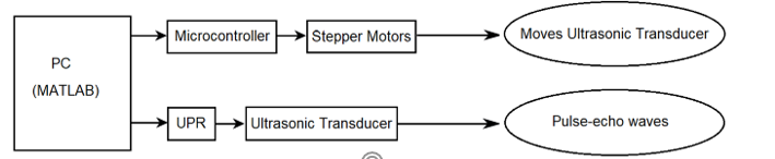Figure 6: Overall Control System

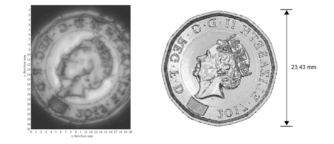Figure 7: Scanned image reads accurate coin dimensions

4. Results and Discussion

To check the applicability and efficiency of this method, the experimental design was performed on a one-pound coin.  The coin was put inside a water tank. The depth of water above the coin was equivalent to the transducer’s focal length of 51 mm. By tracking the amplitude of the ultrasonic pulse, the transducer was then centered on the face of the coin. This process should be done accurately to achieve the best focal spot diameter. A region of 250 mm x 200 mm has been scanned and the image produced is displayed in Figure 7.

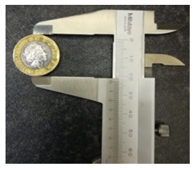Figure 8 Dimensions of the coin as measured by a caliper.

The results reveal that the original coin is clearly mirrored, which confirms the durability of the ultrasonic transducer chosen. The geometry of the coin was examined and linked to the ideal size of the coin as seen in Figure 6. The scanned figure reveals an exterior surface diameter ranging from 23.3 mm to 23.4 mm. This is very similar to the ideal one-pound coin size of 23.43 mm.

To examine the slight size difference, a caliper was used to measure the same coin that was scanned, and the observations are seen in Figure 7. The measurement taken using the caliper have shown that the real coin size is about 23.3 mm in diameter, which is consistent with the readings obtained from our scanning system. This confirms the precision of the 2D motion of the scanner.

Two methods were used to observe the surface profile of the coin. The first approach was based on the intensity of the reflected wave. This follows the theory that was discussed in (2). Figure 9 shows the intensity of the reflected signals from a planar view. Higher intensities were recorded in the middle part of the coin as that area behaves as a better reflector. This is due to the less irregularities in that area, making it similar to a flat reflective surface.

Figure 10 shows the surface profile of the coin which is based on the intensity of the reflected signal. The boundaries of the coin can be easily distinguished through this view. However, the 3D view of the surface profile might require more scaling to be done to replicate the actual surface of the coin.

Figure 11 shows the surface profile of the coin based on the time of signal arrival. It is clear using this figure that the boundaries and 3D profile of the coin can be well observed and appear to be more realistically distributed. This is because the time approach can be easily linked to actual distances when the speed of sound in the given medium is known, as represented in (4).

These results suggest that both the intensity of the reflected signals and the time of their arrivals can be used to obtain useful data from the surface profile. However, it should be noted that the time approach is more commonly used along with an unfocused transducer, which emits all its waves in a parallel direction. The focused transducer emits waves with different inclination angles for focusing, as done in this experiment. Therefore, it is possible to have minor errors in surface readings when this method is used.

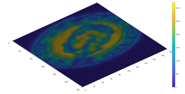Figure 9 Scanned coin based on intensity of the reflected wave

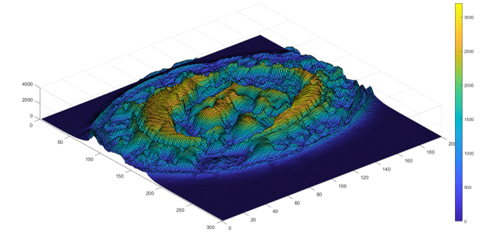Figure 10:The surface profile of the scanned coin based on intensity of the reflected wave

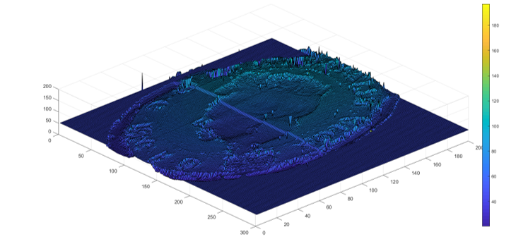Figure 11: The surface profile of the scanned coin based on time of arrival of the reflected wave

Finally, it is important to consider the wave attenuations during the experiments as it can have a great impact on the obtained results. Attenuation coefficient does not depend only on the medium it passes through, but also on the wave frequency. Higher frequencies can result in larger attenuation coefficients. In standing water, the following relation applies to the attenuation coefficient [3]

where a is the attenuation coefficient in dB/m. The relation between both parameters a and f can be shown in Figure 12. The red mark displays the ultrasonic transducer that was used in this experiment and shows an attenuation coefficient of 21.7 dB/m.

By combining both (3) and (5), a relation between focal spot diameter and attenuation coefficient in standing water can be obtained as shown in Figure 13. The signal becomes highly attenuated as the focal spot diameter is decreased. This illustrates one of the main issues of ultrasonic scanning where a reasonable decision should be made when selecting the optimum transducer for the experiment. The optimum case should have a small focal spot diameter to ensure a more accurate reading is obtained. On the other hand, the attenuation coefficient should not be high enough as it might lead to loss of important parts in the signal.

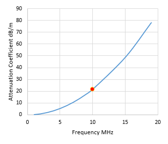Figure 12: Change in attenuation coefficient with Frequency

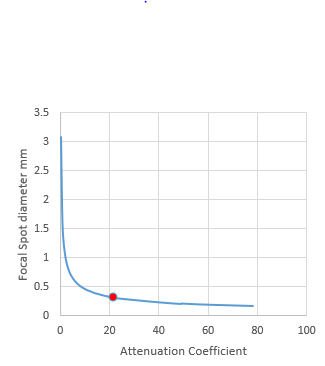Figure 13: Change in focal spot diameter with the attenuation coefficient

5. Conclusion

This paper provides a low-cost approach to the design of a two-dimensional ultrasonic wave scanner. The reliability of this method depends primarily on the transducer’s focal spot diameter and the number of data points collected. Using a high-frequency transducer will improve the focal spot diameter. However, the degree of attenuation should be considered since an inverse relation exists between frequency and attenuation coefficient. This becomes critical when the waves are travelling through materials of higher attenuation coefficient than water.

The total number of collected data points for any scanning operation can be enlarged by reducing the interval distance between two successive datasets. But the total scanning time will significantly increase as the number of scanned data points increase.

A 2D image of a scanned object can be clearly obtained using the intensity of the reflected signals, whereas a 3D image (surface profile) of the same object can be clearly visualized using the time of signal arrival. This scanning approach can be applied to various applications. Future work will utilize this method in measuring the interfacial properties of contacting bodies.

Conflict of Interest

The author declares no conflict of interest.

Acknowledgment

The author acknowledges the support provided by the University of Aberdeen in assembling the experimental setup.

1. F. Aymerich, S. Meili, “Ultrasonic evaluation of matrix damage in impacted composite laminates,” Composites Part B: Engineering, 31(1), 1–6, 2000, doi:10.1016/S1359-8368(99)00067-0.
2. C. Moore, S.B. Promes, “Ultrasound in pregnancy,” Emergency Medicine Clinics of North America, 22(3), 2004, doi:10.1016/j.emc.2004.04.005.
3. H. Krautkrämer Josefand Krautkrämer, Ultrasonic Testing by Determination of Material Properties, Springer Berlin Heidelberg, Berlin, Heidelberg: 528–550, 1990, doi:10.1007/978-3-662-10680-8_34.
4. J.W. Hunt, M. Arditi, F.S. Foster, “Ultrasound Transducers for Pulse-Echo Medical Imaging,” IEEE Transactions on Biomedical Engineering, BME-30(8), 453–481, 1983, doi:10.1109/TBME.1983.325150.
5. K. Bou-Hamdan, “An Experimental Approach that Scans the Surface Area Using Ultrasonic Waves to Generate a Two-Dimensional Image,” in 2020 7th International Conference on Electrical and Electronics Engineering (ICEEE), 264–267, 2020, doi:10.1109/ICEEE49618.2020.9102557.
6. A. Yassin, M.S.U. Rahman, M.A. Abou-Khousa, “Imaging of Near-Surface Defects using Microwaves and Ultrasonic Phased Array Techniques,” Journal of Nondestructive Evaluation, 37(4), 71, 2018, doi:10.1007/s10921-018-0526-9.
7. S.T. Coelho de Souza Padilha, R.G. da Silva Araujo, “New Approach on Cement Evaluation for Oil and Gas Reservoirs Using Ultrasonic Images,” in Latin American and Caribbean Petroleum Engineering Conference, Society of Petroleum Engineers, 1997, doi:10.2118/38981-MS.
8. K.F. Bou Hamdan, R. Harkouss, H.A. Chakra, “An overview of Extended Reach Drilling: Focus on design considerations and drag analysis,” in Mediterranean Gas and Oil International Conference, MedGO 2015 – Conference Proceedings, Institute of Electrical and Electronics Engineers Inc., 2015, doi:10.1109/MedGO.2015.7330328.
9. F. Aymerich, M. Pau, F. Ginesu, “Evaluation of Nominal Contact Area and Contact Pressure Distribution in a Steel-Steel Interface by Means of Ultrasonic Techniques.,” JSME International Journal Series C, 46(1), 2003, doi:10.1299/jsmec.46.297.
10. K. Hodgson, R.S. Dwyer-Joyce, B.W. Drinkwater, “Towards an ultrasonic mapping of the contact pressure within an engineering component,” in Tribology Series, Elsevier: 79–85, 2001, doi:10.1016/s0167-8922(01)80095-x.
11. W. Lowrie, A. Fichtner, Fundamentals of Geophysics, Cambridge University Press, 2020, doi:10.1017/9781108685917.
12. K.I. Maslov, L.M. Dorozhkin, V.S. Doroshenko, R.G. Maev, “A new focusing ultrasonic transducer and two foci acoustic lens for acoustic microscopy,” IEEE Transactions on Ultrasonics, Ferroelectrics, and Frequency Control, 44(2), 380–385, 1997, doi:10.1109/58.585122.
13. T.E. Gómez Álvarez-Arenas, J. Camacho, C. Fritsch, “Passive focusing techniques for piezoelectric air-coupled ultrasonic transducers,” Ultrasonics, 67, 85–93, 2016, doi:10.1016/j.ultras.2016.01.001.
14. M.T. Balmaseda, M.T. Fatehi, S.H. Koozekanani, A.L. Lee, “Ultrasound therapy: A comparative study of different coupling media,” Archives of Physical Medicine and Rehabilitation, 67(3), 1986, doi:10.1016/0003-9993(86)90052-3.
15. P. Acevedo, M. Fuentes, J. Durán, M. Vázquez, C. Díaz, “Pulse Generator for Ultrasonic Piezoelectric Transducer Arrays Based on a Programmable System-on-Chip (PSoC),” Advances in Science, Technology and Engineering Systems Journal, 2(3), 2017, doi:10.25046/aj020327.

(Click Here)