1. Introduction

Currently, agriculture continues to modernize and follow the evolution of new technologies to improve production practices and crop management. That has become a need in many countries due to the increasing demand for food. The use of new technologies, such as Unmanned Aerial Vehicle (UAV), can help find solutions and add value to several agricultural problems, thus promoting productivity, better quality control processes and flexible tree management [1]. Additionally, strategies that allow data analysis from agricultural environments, including artificial vision systems, can help optimize current practices, such as crop counting, yield estimation, diseases detection and classification of crop maturity [2]. Information on the number of plants in a crop field is essential for farmers as it helps them estimate productivity, assess the density of their plantations and errors occurring during the planting process [3]. From a perspective of detection, delimitation and counting of trees and in particular fruit trees, in [4] the author developed and tested the performance of an approach, based on RGB UAV imagery, to extract information about individual trees in an orchard with a complicated background which includes apple and pear trees. In [5], the author proposed an efficient method for an individual trees segmentation and the measurement of the width and area of identified trees crowns, based on images acquired by RGB UAV camera. The collected images from a peach orchard in Okayama, Japan, were integrated into Pix4Dmapper software for processing and generation of derived products (Digital Surface Model DSM). Using the intersection of the polygons corresponding to the peach branch line with the summer season DSM as markers indicating the sources of flooding, authors were able to delineate the peach trees crown via watershed segmentation. In [6], the author developed a specialized approach for citrus detection based on the DSM extraction. In [7], the author applied the Canny filter for edge detection applied to the images followed by the “Circular Hough Transform CHM” algorithm thus achieving the extraction and delineation of citrus trees.

The use of UAV in various arboriculture applications has many advantages and benefits. However, this depends on the types of sensors, mission objectives and their platforms [8], [9]. Nevertheless, there are some problems that need to be considered when using UAV such as the reliability of the platform, sensor capacity and adequate treatment of the images [10]-[12]. To solve the problem of image processing which presents a main source of the success of predictions or good estimation, researchers have in recent years turned to artificial intelligence algorithms, particularly deep learning and especially the convolutional neural network. In [13], the author evaluated the use of convolutional neural network (CNN) -based methods for the detection of legally protected tree species. Three detection methods were evaluated: Faster R-CNN, YOLOv3 and RetinaNet. In [14], the author proposed a deep learning method to accurately detect and count bananas. In [15], the author exploited convolutional neural networks for the detection and enumeration of citrus fruits in an orchard in Brazil characterized by the high density of its trees. In [16], the author developed an automatic strawberry flower detection and yield estimation system.

Following the state of art review, we have selected some of efficient CNN architectures that we have implemented and tested on our context and data. The second phase is the preparation of the data especially the collection, cleaning, analysis, visualization and necessary treatments. The third phase consist to conceive, implement and analysis of the models performance. One of our objectives is to understand the advantage of one architecture over another. We have started by testing different architectures and their hyperparameters. The knowledge acquired as a result of these experiments allowed us to understand the influence of several parameters on the expected performance and to subsequently build a model intended to detect fruit trees.

The rest of this paper is organized as follow. Section 2 gives the material and the used methods.  The experimental results and setup are shown in section 3. Section 4 presents the result discussion and section 5 the conclusion followed by the most relevant references.

2. Material and Methods

2.1. Material

2.1.1. Data collection

Among the many challenges of deep learning algorithms is the data collection which is considered to be one of the most critical points in the processes of artificial intelligence in general and deep learning in particular. The required time to run a deep learning algorithm depends on data preparation including collection, cleaning, analysis, and visualization. To answer this problem, we consulted several sources, resulting in a fairly large repertoire of images serving as the basis for feeding our algorithm. In this work, we will not treat the acquisition step and orthophoto establishment. We are limited in their uses and treatment for a successful training operation.

We present in Table 1 the number and size of each of the data acquired as well as the source.

Table 1: The number, size and source of data tested in this study

Data	Ima-ge num-ber	Size	Camera resolu-tion MPx	Alti- tude	Type of flight	Source
D1	103	960 x 540	–	–	–	https://github.com/skygate/skyessays
D2	170	400 x 400	–	–	–	(http://data.neonscience.org/
D3	1	9649 x 4532	20	120	Ebee sensefly	www.etafat.ma
D4	17	5472 x 3846	18.6	80	Ebee	Globetude company
D5	13	4896 x 3672	16	40	DJI	www.terramodus.ma

2.1.2. Computer tools and deep learning libraries used

Keras

Keras is a high-level neural network Application Programming Interface (API) written in Python and interfaceable with TensorFlow, CNTK and Theano. It was developed with the aim of allowing rapid experiments [17]. Keras can allow rapid and easy prototyping (due to its user-friendliness, modularity and extensibility). It supports both convolutional networks and recurrent networks as well as a combination of the two. Also, it Works seamlessly on CPU and GPU.

Darknet

Darknet is an open source neural network framework written in C and CUDA. It is fast, easy to install, and supports CPU and GPU computing [18]. It was developed by Joseph Redmon. Unlike Keras which is well known as much as a deep learning library, Darknet on the other hand is the library where versions of the YOLO object detector are implemented.

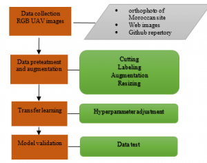
Figure 1. Methodology flowchart.

Google colaboratory

For any neural network, the training phase of the deep learning model is the most resource-intensive task. During training, a neural network receives input data, which is then processed in hidden layers using weights which are adjusted during training and the model then gives a prediction. The weights are adjusted to find patterns to make better predictions. Memory in neural networks is needed to store input data, weight parameters, and activations as an input propagates through the network [19]. Due to the memory and limited power of our computer, we used the Google colaboratory to perform all of our deep learning operations. Google Colab or Colaboratory is a cloud service, offered by Google (free), based on Jupyter Notebook and intended for training and research in machine learning. This platform allows you to train machine learning models directly in the cloud (Google Colab: The Ultimate Guide). Colab provides a free Tesla K80 type GPU graphics processor and 13 GB of random-access memory (RAM) that work entirely in the cloud.

2.2. Methods

Our methodology is based on a following processes as presented in figure 1.

In the following sections we develop the methodology process.

2.2.1. Cutting operation

In order to increase the images number for the algorithm training, a cropping operation was performed on large images as well as the orthophoto. This operation consisted of splitting the original image to smaller images with a dimension of 816 x 816 pixels, the number of images resulting from the trimming operation depends on the initial dimensions of the image. This was done using the OpenCV image processing graphics library on Python. Figure 2 shows how an image of dimension 4 x 4 is divided into images of dimension 2 x 2.

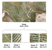
Figure 2: Cutting the orthophotographie using OpenCV algorithm

2.2.2. Labeling of images

Labeling images is a human task that involves annotating an image with labels. These labels are predetermined by the person and are chosen to give the computer vision model information about what is shown in the image. The tool used for this task is LabelImg. This is a graphical image annotation tool, it is written in Python and uses for its GUI. Annotations are saved as XML files in Pascal VOC format, the format used by ImageNet. Besides, it also supports YOLO format.

2.2.3. Image augmentation

One of the main difficulties in training a CNN model is that of overfitting. That is, the model produced fits too well on the training data. But, therefore the generalization error of the model is much too high, in other words the model modifies its predictions based on the size, angle and position of the image. To deal with the over-adjustment problem, several techniques are used and among them: Dropout, Transfer learning, Batch normalization and data augmentation. Unlike the techniques mentioned above, increasing the data resolves the problem from its origin, namely the training data set. This is done on the assumption that more information can be extracted from the original dataset through augmentation. Data augmentation is the technique of increasing the size of the data used to train a model. To obtain reliable detection, deep learning models often require a lot of training data, which is not always available. Therefore, the existing data is augmented in order to obtain a better generalized model. Some of the most common data augmentation techniques used and applied to our images are listed below: Scaling, Rotation, Translation, Shear, Brightness, Contrast, Saturation, Hue, Noise, and Blur the image. Figure 3 presents some criteria used in the augmentation phase.

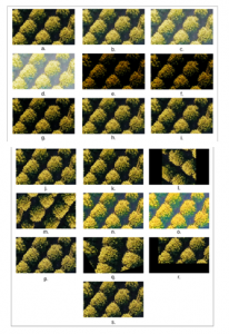
Figure 3: Augmentation algorithm by change of image pixel value : (a) initial image. (b) brightness γ = 1.5. (c) brightness γ = 2.5. (d) brightness γ = 5. (e) brightness γ = 0.3. (f) brightness γ = 0.4. (g) brightness γ = 0.7. (h) Gaussian Blur = 2. (i) Gaussian Blur = 1. (j) Average Blur. (k) Median Blur. (l) rotation θ = 90 °. (m) rotation θ = 180 °. (n) saturation = 50. (o) saturation = 100. (p) Sharpen. (q) Shear. (r) translation. (s) noise.

2.2.4. Resizing training images

We opted to resize the training images because there is a correlation between the dimensions of the images used for training the model and the RAM size needed for the model training. The dimensions chosen for the images training are 416 x 416 and 608 x 608. By resizing the images, all the annotation files must be adapted to the new dimensions of the images so that each enclosing rectangle drawn during the annotation phase remains placed around the object. For this task, the algorithm used is written in python using the OpenCV library.

2.2.5. CNN models used for fruit trees detection

Considering the huge set of applications for the object detection, a very large number of models suitable has been introduced. In what follows, we present the three models chosen for the realization of our work. To make our choice, we are based on the model’s performance as well as on the models used for our similar application. The three models chosen are:

• YOLOv4
• YOLOv3
• RetinaNet-101

YOLO, You Only Look Once, is a real-time object detection system that recognizes various objects in a single enclosure. In addition, it identifies objects faster and more accurately than other recognition systems [20]. A modern detector is generally made up of two parts, a “backbone” part of the detector which is pre-trained on ImageNet and a Head which is used to predict the classes and limit boxes of objects. For detectors running on a GPU platform, their base network can be VGG, ResNet, ResNeXt, or DenseNet. For detectors running on a CPU platform, backbone can be SqueezeNet, MobileNet or ShuffleNet. As for the main part of the detector head, it is generally classified into two categories, namely the single stage object detector and the two-stage object detector. The most representative two-stage object detector is the R-CNN series, which includes Faster R-CNN, R-FCN and R-CNN Libra. For the one-step object detector, the representative models are YOLO, SSD and RetinaNet.

YOLOv4 network implements CSPDarknet53 as the backbone network. YOLOv4 is considering a few options for the neck, including: FPN, PANet, NAS-FPN, BiFPN, ASFF, SFAM. Neck components generally flow from top to bottom between layers and connect only a few layers at the end of the convolutional network. As part of this work, we chose PANet for the aggregation of network characteristics whose efficiency has been approved by the authors [21]. In addition, we have added an SPP block after CSPDarknet53 to increase the receive field and separate the most important features of the backbone.

YOLOv3 addresses object detection as a problem of direct regression from pixels to the coordinates of bounding rectangles and class probabilities. The input image is divided into S × S tiles. For each bounding rectangle, an objectivity or confidence score is predicted by logistic regression, which indicates the probability that the bounding rectangle in question has an object of interest. In addition, the probabilities of a class C are estimated for each bounding rectangle, which indicates the classes it may contain. In our case, each bounding rectangle can contain a fruit tree or the background (interesting object). Thus, each detection in YOLOv3 is composed of four parameters for the bounding rectangle (coordinates), an objectivity or confidence score and class C probabilities. To improve the precision of detection, YOLOv3 predicts these bounding rectangles at three different scales using the idea of setting up a network of pyramids. As a backbone network YOLOv3 uses Darknet-53.

RetinaNet is a single stage object detector similar to YOLOv4 and EfficientDet. However, unlike these two detectors presented previously and which both recent (2020), RetinaNet on the other hand was introduced in 2018. It is based on the ResNet network which makes it possible to add a connection connecting the input of a layer with its release. In order to reduce the number of parameters, ResNet does not have fully connected layers. GoogleNet and ResNet are much deeper but contain fewer parameters. This can make them more expensive in memory during training.

2.2.6. Hyperparameters selection

Several hyperparameters have been tested and iterated by empirical tests. We present in what section the hyperparameters whose variation has remarkably influenced the detection results rate.

The epochs number, stages per epoch and the size of the batch

Epoch’s number is a hyperparameter that defines the number of times the training algorithm will work through the training data set. The size of the batch is a hyperparameter which defines the number of samples to be processed before updating the internal parameters of the model. The number of samples reviewed in a single epoch is set simultaneously based on the number of steps per epoch and the batch size. For example, taking a batch size of 32 and a number of steps of 1000 per epoch, then the number of the network samples worked on is 32000.

Learning rate

Considered to be the most important of all hyperparameters. If it is too low the convergence is slow, if it is too large the gradient descent algorithm may unintentionally increase the training error rather than decrease it.

Subdivisions Number

This is a specific hyperparameter to YOLO models and which allows the batch to be subdivided into mini batches which will be supplied to the machine during training. For example, a batch size of 64 and a number of subdivisions 16 means that 4 images will be loaded at the same time. It will take 16 of these mini batches to perform a full iteration. For all the hyperparameters, several values were tested for each of the models and on the basis of the performance obtained on the validation data that we validate the best hyperparameters for each of the models. Table 2 presents the hyperparameters values tested during training phase.

Table 2: The hyperparameters values tested during training phase

Hyperparameters	Tested value
Epochs number	Variable according to training time
Learning rate	0.01, 0.001, 0.0001, 0.00001
Subdivisions Number	16, 8

3. Results and experimentation

3.1. Data Preparation Results

The augmentation operation allowed us to have, from a limited number of images, a very large set. We distributed the images obtained respectively into training image, validation image and test image as presented in table 3.

Table 3: Distribution of images on the training, validation and test sets

Set	Training	Validation	Test
Rate	80%	10%	10%
Total number of images	2355	263	266
Tree number	140293	17605	24637

The size of the adopted images depends on the network size and the GPU capacity (graphics card) used for training. You must insert a reasonable size batch into the GPU memory. We did some tests with different images sizes. Then we compared the details obtained for the different sizes and the training time to finally choose the most suitable one. The dimensions of images used for training the models are 416 x 416 and 608 x 608. These dimensions are multiples of 32 since YOLO is designed in such a way that the input images for its training have this characteristic.

3.2. Model training and hyperparameters choice

The goal during the training phase is to minimize the loss function. The optimization algorithm used during this work is that of the gradient descent applied to batches (Mini-batch gradient descent). This method updates the weights for each batch consisting of N training samples. At each iteration, we therefore take a batch. It is said that an epoch has passed after the entire dataset is covered. The number N of samples in a batch represents another hyperparameter to be adjusted. During training, there are several choices available with respect to the sizes of the hyperparameters. These are the parameters whose value are set before the start of the learning process. They cannot be learned directly from data and must be predefined. Unfortunately, there is no generic way to determine the best hyperparameters. The optimization or modification of hyperparameters is the major problem for training our model. The same model with different choices of hyperparameters can generalize different data models. Additionally, the same type of machine learning model may require different constraints, weights, or learning rates to generalize different data models. So we experimented with different values of these parameters including the learning rate, the batch size and the network architecture. We train our model and at the end we choose the parameters that provide the best precision. Table 4 shows the values taken from the hyperparameters to reduce the loss function.

Table 4: the list of the different pre-trained models and their hyperparameters

Model	Basic network	Image size	learning rate
RetinaNet 101	ResNet 101	608	0.00001
YOLOv4	CSPDARKNET53	416	0.001
YOLOv3	DARKNET53	416	0.001

The loss function of training data is plotted over time. We start with the RetinaNet architecture by referring to the hyperparameters presented in Table 4. Figure 4 presents the evolution of loss functions by epoch

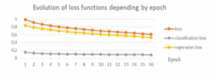
Figure 4: The evolution of loss functions by epoch.

We notice a decrease in the loss function. The experienced learning rate is 0.00001. We also observe that the loss function for the classification has a lower value compared to the other two. This is explained by the fact that we only have one class which is fruit trees.

Unlike RetinaNet which is executed using the Keras library and which allows to visualize the progress of the loss function during the training using the tenserboard module, with Darknet (base network of YOLOv3 and YOLOv4) the progress of the training is not recorded. Nevertheless, we were able to visualize his progress during the training.

For the YOLOv3 model, we could not complete training for a frame size of 608 due to the size of the RAM. We were satisfied with images of dimensions 416 x 416 for the training. Furthermore, it was possible to use a larger batch size for YOLOv3 such as 64. This is made possible thanks to a hyperparameter called subdivision. The smaller the number of subdivisions, the faster the training and the more memory it requires. For example, a number of subdivisions of 8 means that 8 images will be loaded at a time, so more memory will be consumed. For us, the number of subdivisions that can support our work environment is 16 that is mean to load 4 images at once for a batch size of 64. Table 5 shows the values of the loss function of the YOLOv3 model.

Table 5: Values of the loss function at the start and the end of learning- YOLOv3.

Model	Batch size	Subdivision Number	Loss at the start of learning	Loss at the end of learning for 5000 iterations
YOLOv3	64	16	2500	3.67

The results of the YOLOv4 model will be presented in a similar way to those of YOLOv3. Unlike YOLOv3, the training for YOLOv4 has been done up to 10000 iterations mainly because the training speed is much faster compared to YOLOv3. Similar to YOLOv3, YOLOv4 is run using DarkNet and not Keras. Thus, we cannot obtain at the end of the training the progress of the latter. However, we can get an idea of the behavior of the loss function. This function has been tested with a learning rate of 0.001 and 0.0001. This decrease is much faster with a learning rate of 0.001.  Table 6 presents the values of the loss function of YOLOv4.

Table 6: The values of loss function at the start and the end of learning- YOLOv4

Model	Batch size	Subdivision Number	Loss at the start of learning	Loss at the end of learning for 5000 iterations
YOLOv4	64	16	2800	12.5624

3.3. Detection rate for the 3 architectures

As test data, we will use the 10% of the images reserved for this step. Figure 5 shows the detection results:

From the detection result, we can see that the two models YOLOv3 and YOLOv4 give better predictions. In addition, the RetinaNet model fails to give good detections of trees if the number of trees in the images is very small. Table 7 presents the predictions of tree number detection in UAV images:

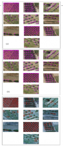
Figure 5: Example of detection results: (a) YOLOv4, (b) YOLOv3, (c) RetinaNet101.

Table 7: The detections obtained for the three tested models

Model	Detection rate %
RetinaNet-101	73%
YOLOv3	80%
YOLOv4	96%

The results obtained demonstrate that the YOLOv4 model is the model which gave the best validation and test results.

The reasons for this choice are as follows:

• Yolov4 allowed a faster improvement of the loss function compared to other architectures. For the same number of epochs, this reaches its lowest value. In addition, it does not require a lot of time for training.
• Yolov4 is the model which sacrifices the least precision to improve its Recall.
• Yolov4 provides very satisfactory results on the test set where it gives better detections with minimum time and better detection speed.

4. Discussion

Fruit trees have a very complex and heterogeneous form with vegetation classes that appear visually similar in orchards. Their categorizations require the detection model to be able to represent the spatial context of the image appropriately by learning a set of attributes adequate to distinguish between the different categories of the agricultural scene and the efficient extraction of fruit trees. Such an analysis is often carried out on images with very high spatial resolution and which have sufficient detail. Hence the considerable contribution of using RGB UAV images for the detection and enumeration of fruit trees.

The proposed approach based on the Yolov4 model that we implemented, succeeded in identifying and counting these trees. The results obtained on the validation and test sets are very satisfactory, it gave an accuracy of 96%. In addition, the results on various evaluation metrics undoubtedly confirm the contribution of convolutional neural networks algorithms. Despite their good performance, the use of convolutional neural networks presents challenges, the most important of which is the recurrent risk of overfitting. CNNs are big consumers of data. The general rule of learning algorithms is that a model trained on a large amount of data produces, in the majority of cases, much better results on new data than a model trained on small amounts. The amount of data required is not fixed and depends closely on the complexity and the mission objective.

Finally, despite the relevance of the obtained results, our work nonetheless presents some limitations which are most often due to the available computing resources which have proved insufficient for the conduct of some experiments. In recent years, the graphics processor (GPU) has established itself as an important and even indispensable player in heavy calculations that have long been done only by central processors (CPUs). Fortunately, the Google colaboratory cloud space offers excellent technical specifications and allowed us to run several experiments related to this work. Furthermore, we cannot present an experiment that takes place over a succession of stages without addressing the notion of time. Time is one of the deciding factors in choosing the best architecture. Of course, while weighting with the detection rate obtained. Table 5 presents a comparison of the overall training time for the three tested models.

Table 5: The overall training time for the three tested models

Model	Overall training time
RetinaNet-resnet101	11h
Yolov3	5h
Yolov4	8h08min

According to table 5, it can be seen that the Yolov3 and yolov4 model require less time than the Retinanet-101 model. Also the Yolov3 model consumes less time in the training phase. However, as we have mentioned before. Time cannot be the only parameter in the choice of the model. It will be necessary to weight according to the precision of detection. In this sense, Yolov4 allowed us to obtain the best precision in a fairly satisfactory time.

5. Conclusion

We have tried to simplify the various experiments carried out either on the hyperparameters or on the architectures obtained. Our main goal is to obtain good details on the fruit tree detection and counting. This was accomplished with a detection success to 96%. These results are generally satisfactory given the difficulties encountered either in the availability of data or in the implementation of architectures. During this work, a considerable amount of time is spent for data preparation, collection, cleaning, analysis, visualization and the necessary treatments namely resizing, augmentation and annotation. Our primary concern is to find a sufficient number of images of fruit trees taken by UAV and which can be used subsequently to train, validate and test by the deep learning algorithm. In addition, the field of deep learning is constantly evolving and requires having solid basic knowledge and keeping up with all the news. Something that slowed down our work and took a long time for us to resolve implementation errors. Finally, the complexity of the calculations generated by the different models always makes their training requires more time and powerful machines. In conclusion, despite all these difficulties, it emerges that convolutional neural networks are very promising for the detection and enumeration of fruit trees and open a very interesting field of application for other uses such as yield estimation.

1. K. R. Krishna, “Agricultural drones: A Peaceful Pursuit,”1e edition Editions Apple Academic Press, Inc. USA & Canada, 2018.
2. J. P. Vasconez, J. Delpiano, S. Vougioukas, F. Auat Cheein, “Comparison of convolutional neural networks in fruit detection and counting : A comprehensive evaluation,” Computers and Electronics in Agriculture, 173, 105348, 2020, doi:10.1016/j.compag.2020.105348.
3. Y. Ampatzidis, V. Partel, “UAV-Based High Throughput Phenotyping in Citrus Utilizing Multispectral Imaging and Artificial Intelligence, ” Remote Sens., 11(4), 410, 2019, doi:10.3390/rs11040410.
4. X. Dong, Z. Zhang, R. Yu, Q. Tian, X. Zhu, “Extraction of information about individual trees from high-spatial-resolution UAV-acquired images of an orchard,” Remote Sensing, 12(1), 133, 2020, doi:10.3390/rs12010133.
5. Y. Mu, Y. Fujii, D. Takata, B. Zheng, K. Noshita, K. Honda, S. Ninomiya, W. Guo, “Characterization of peach tree crown by using high-resolution images from an unmanned aerial vehicle,” Horticulture Research, 5(1), 1–10, 2018, doi:10.1038/s41438-018-0097-z.
6. A.O. Ok, A. Ozdarici-Ok, “2-D delineation of individual citrus trees from UAV-based dense photogrammetric surface models,” International Journal of Digital Earth, 11(6), 583–608, 2018, doi:10.1080/17538947.2017.1337820.
7. D. Koc-San, S. Selim, N. Aslan, B.T. San, “Automatic citrus tree extraction from UAV images and digital surface models using circular Hough transform,” Computers and Electronics in Agriculture, 150, 289–301, 2018, doi:10.1016/j.compag.2018.05.001.
8. A.C. Watts, V.G. Ambrosia, E.A. Hinkley, “Unmanned aircraft systems in remote sensing and scientific research: Classification and considerations of use,” Remote Sensing, 4(6), 1671–1692, 2012, doi:10.3390/rs4061671.
9. S. Nebiker, A. Annen, M. Scherrer, D. Oesch, “A light-weight multispectral sensor for micro UAV—Opportunities for very high resolution airborne remote sensing,” Int. Arch. Photogramm. Remote Sens. Spat. Inf. Sci, 37(B1), 1193–1200, 2008.
10. C. Zhang, J.M. Kovacs, “The application of small unmanned aerial systems for precision agriculture: a review,” Precision Agriculture, 13(6), 693–712, 2012.
11. A.S. Laliberte, A. Rango, J.E. Herrick, “Unmanned aerial vehicles for rangeland mapping and monitoring: a comparison of two systems,” in ASPRS Annual Conference Proceedings, 2007.
12. P.J. Hardin, T.J. Hardin, “Small-scale remotely piloted vehicles in environmental research,” Geography Compass, 4(9), 1297–1311, 2010, doi:10.1111/j.1749-8198.2010.00381.x.
13. A.A. dos Santos, J. Marcato Junior, M.S. Araújo, D.R. Di Martini, E.C. Tetila, H.L. Siqueira, C. Aoki, A. Eltner, E.T. Matsubara, H. Pistori, “Assessment of CNN-based methods for individual tree detection on images captured by RGB cameras attached to UAVs,” Sensors, 19(16), 3595, 2019, doi:10.3390/s19163595.
14. B. Neupane, T. Horanont, N.D. Hung, “Deep learning based banana plant detection and counting using high-resolution red-green-blue (RGB) images collected from unmanned aerial vehicle (UAV),” PloS One, 14(10), e0223906, 2019, doi:10.1371/journal.pone.0223906.
15. M. Zortea, M.M.G. Macedo, A.B. Mattos, B.C. Ruga, B.H. Gemignani, “Automatic citrus tree detection from uav images based on convolutional neural networks,” in 2018 31th SIBGRAPI Conference on Graphics, Patterns and Images (SIBGRAPI), 2018, doi:10.3390/s19245558.
16. Y. Chen, C. Hou, Y. Tang, J. Zhuang, J. Lin, Y. He, Q. Guo, Z. Zhong, H. Lei, S. Luo, “Citrus tree segmentation from UAV images based on monocular machine vision in a natural orchard environment,” Sensors, 19(24), 5558, 2019, doi:10.3390/s19245558.
17. A. Gulli, S. Pal, Deep learning with Keras, Packt Publishing Ltd, 2017.
18. S.R. Masurkar, P.P. Rege, “Human Protein Subcellular Localization using Convolutional Neural Network as Feature Extractor,” in 2019 10th International Conference on Computing, Communication and Networking Technologies (ICCCNT), IEEE: 1–7, 2019, doi:10.1109/ICCCNT45670.2019.8944812.
19. T. Carneiro, R.V.M. Da Nóbrega, T. Nepomuceno, G.-B. Bian, V.H.C. De Albuquerque, P.P. Reboucas Filho, “Performance analysis of google colaboratory as a tool for accelerating deep learning applications,” IEEE Access, 6, 61677–61685, 2018, doi:10.1109/ACCESS.2018.2874767.
20. A. Bochkovskiy, C.-Y. Wang, H.-Y.M. Liao, “Yolov4: Optimal speed and accuracy of object detection,” ArXiv Preprint ArXiv:2004.10934, 2020.
21. D. Wu, S. Lv, M. Jiang, H. Song, “Using channel pruning-based YOLO v4 deep learning algorithm for the real-time and accurate detection of apple flowers in natural environments,” Computers and Electronics in Agriculture, 178, 105742, 2020, doi:10.1016/j.compag.2020.105742.

(Click Here)