1. Introduction

This paper is an extension of work originally presented in SNPD2019 [1] by the further detail data analysis and algorithm explanation. It has been widely known that the decrease of nerve cells and the deterioration of cognitive function in accordance with aging can cause the deterioration of memory, thinking, and motivation [2]. As the symptoms of dementia, cerebral disorder is also known, e.g. memory impairment, judgment disorder, execution function disorder, dropping off of cognitive ability, etc. It has also been shown that the older people get, the higher the possibility of the occurrence of disease. In the case of dementia patients, a depressing symptom deprives him/her of vitality and even interest in what he/she used to be interested in before.

Doctors mainly determine whether dementia occurs on the basis of medical diagnostic criterion. Dementia can be classified into several types such as Alzheimer dementia, dementia with Lewy bodies (DLB), etc. Early diagnosis enables the specification of disease and appropriate prognosis treatment. However, there are not a few cases where temporal, economic, and geographical difficulties might obstruct early diagnosis by doctors.

It has been known that the deterioration of brain function can cause the impairment of consumption activity, such as being unable to withdraw money from banking facilities or to do shopping in spite of ample money. The case of increasing savings without using money because of abnormal adherence to money is also one form of declining consumption activity as well.

The relationships have been revealed between the deterioration of cerebral function and the reduction of consumption activity of elderly people. The malfunction of cerebral function advances if not treated properly or immediately, and can disrupt even daily life owing to dementia, etc.

For the single elderly person, existing techniques enable us to determine dementia by their behaviors in their daily lives. For example, a system has been developed that predicts dementia by using input information in order to inform and input their safety [3]. This system can observe the safety under the protection of the elderly’s privacy as well as foresee dementia without regular medical check-ups. Another system is a household electric appliance that determines if the operator is possibly experiencing dementia by obtaining his/her operation history, sleeping hours, commodity purchase history, etc. [4]. If the possibility of dementia is determined, the information is sent to an external device owned by the family of the operator. However, it would be indispensable to monitor the behavior of elderly people to determine if he/she has dementia. Therefore, it would be necessary to purchase the devices and install them to monitor him/her.

The jeopardies of economic activity ability are classified into the following two types: (1) “Dissaving risk,” including the possibility of being victimized by fraudulent means, which results from the impairment of judgement, etc., (2) “Under-consumption risk” that is caused by the lowering of motivations. Therefore, the objective of our work is to develop a system that detects those jeopardies early on and issues a warning. In this paper, “dissaving risk” is focused on.

So far we have employed anonymous data (AD) on the basis of the National Survey of Family Income and Expenditure (NSFIE) [5] conducted by Ministry of Internal Affairs and Communications (MIC) in 2004. As a basis of economy activity, for the data of single households at the age of sixty-five or older, clustering was performed with five clusters based on income and saving [6]. As a result of analysis, five clusters were obtained and characteristically classified. Then we developed a method to determine if savings are enough against life expectancy in terms of income and savings [6]. The analysis results revealed that correction detection ratio of the data determined as dissaving risk ranged from 52.6 to 94.1%.

Nevertheless, our first method showed the limitations with the additions of AD years 1994 and 1999. Therefore, our second method has been proposed with a view to determining immediately and easily cerebral function that has started to decline by focusing on economical ability of single-person and two-person households at the age of sixty-five or older [7]. Here, the analysis data were divided into test data and training data [7]. Then two-step methods were then taken to determine dissaving risk [7]. Three kinds of methods were performed in terms of income and savings. However, the security of anonymity for AD could be controversy [1]. In addition, AD can be available and must be returned within the designated durations after application is approved [8]. In order to reinforce the anonymity of AD, random data (RD) is generated along with AD and then compared with the previous analysis [7], for the purpose of performance evaluation. The analysis result conveys the conclusion that using the RD might be as effective as using mere AD [1] in evaluating the performance of the proposed method [7].

In our previous paper [1], the analysis methods and results were superficially and briefly summarized due to space limitations. Therefore, this paper provides more detailed analysis methods and results so that our proposed method [7] would be understood more profoundly.

The remainder of the paper is organized as follows. Related works are referred in Section 2. Preparation of the analysis is summarized in Section 3. The outline of our proposed method [7] using AD is explained in Section 4. Analysis results using RD to evaluate the proposed method [7] is explained in Section 5. Finally, Section 6 concludes the paper.

2. Related Works

In [9], authors pointed out that the shrink of economic activity of rapidly increasing dementia patients along with aging could influence actual economy. For example, when an elderly person develops dementia, he/she might repeat the following experiences; he/she is unable to withdraw money from his/her bank account because of not remembering password, forgets to pay bills, repeatedly purchases what he/she already had before. These experiences could result in considerable reduction of economic activities. On 2012 fiscal year, among the elderly people at the age of sixty-five or older, the number of dementia patients is approximately 4.62 million, while that of mild cognitive impairment (MCI) attains roughly 4 million [9]. The sum of these patients account for close to 7% of Japanese. Since the elderly people occupy most portions of dementia patients, their figure is expected to go on increasing on a global scale in the upcoming several decades [9]. Thus the shrink of economic activities will extremely impact on economy worldwide. From these viewpoints, our work focuses on the possible decline of economic activities of the elderly people.

In [10], authors conducted an experiment with a view to investigation on annual change of economical ability related to variation from MCI to dementia [10]. They managed the subjects on financial capacity instrument (FCI) under one-year follow-up. The subjects are composed of the following three types: 76 Controls, 25 MCI Converters, and 62 MCI Non-Converters; Control is healthy elderly people, whereas MCI Converter (MCI Non-Converter) is a subject on whom the inflection from MCI to Alzheimer-type dementia was (was not) observed. Using multivariate analysis of variance (MANOVA), the performance of FCI domain and global scores are compared within/among groups. As a result of analysis, MCI Converters fell short of MCI Non-Converters, from the viewpoints of economical concepts, money withdraw management of bank deal specification, payment on invoice, and total FCI scores. Although this research indicates the degradation of economic activities themselves of MCI patients, it is not based on actual consumption behaviors.

In [11], the authors researched on money management issues of the elderly people households along with aging and cognitive ability deterioration. In [12], the authors investigated if the knowledge of basic concepts necessary for effective and economical choice would be degraded after sixty years old, for the purposed of detecting the evidence of intelligence decline in accordance with aging that influences the ability necessary for money management. In [13], the authors analyzed the impact of information against cognitive ability decline of decision maker of finance by using time-series data related to elderly married couples. Authors made an analysis on cognitive ability by employing the actual examples of almost best behaviors and ample economic decisions of consumers. Analysis results conveyed the conclusion that consumers with overall higher scores on analysis items and mathematics are unlikely to end up with economic collapse. These researches [10-13] have been analyzed on the basis of anecdotal reports and multiple manifold methods such as regression analysis. Nevertheless, there have been no researches that focus on the relationships between cognitive ability and purchase motivation.

In [14], the authors evaluated default risks through comparing transition of representative financial ratio considered as the financial safety of companies among bankrupt firms and non-bankrupt firms. For financial ratio, fourteen feature values are extracted; four for profitability and ten for security. These fourteen time-series variation  of financial ratio were described to investigate the validity of financial ratio analysis in default risk evaluation. This research analyzes bankrupt risk for enterprises. However, no indications for individual bankrupt risk were referred.

In [15], the authors used AD to study on relationships between living expenses and fortunes for medical care risks by classifying family budgets, e.g. higher income, lower income, and so on. It has been suggested that appropriate household plans are possible that foresee life cycle of “how much savings will be able to keep covering anticipated household expenditure.”

3. Preparation for Analysis

3.1.  Anonymous Data (AD)

The analysis data employed for our previous works [1,6,7] is an AD obtained from National Statistics Center (Japan) [16], based on NSFIE carried out by MIC in 1994, 1999 and 2004. This data contains 1,919 (1,752 and 1,780, respectively) detailed family income and expenditure survey items for 1994 (1999 and 2004), e.g. the amount of income and expenditure, expenditure amount of food such as crop, fish, meat, etc. Among the AD, the present paper uses the data of single elderly people and two-person households (Twos) at the age of sixty-five or over; 717 single males, 3,475 single females, and 11,528 two-person households. There are two types of Twos; head of household is either male or female. However, the Twos whose head is male (1994: 2,607, 1999: 3,840, 2004: 5,081, total: 11,528) considerably outnumbers those whose head is female (1994: 20, 1999: 39, 2004: 44, total: 103). Thus, the Twos whose head is male are used for the analysis data.

3.2.  Revised Disbursement

Disbursement consists of the following three components: (1) Expenditure, (2) Disbursements other than expenditure, and (3) Carry-over to next. Among the disbursement, the items that should be exempted from disbursement were considered [6]. As a result, five items were determined to exclude from disbursement [6]; saving, insurance premium payments, security purchase, property purchase and carry-over to next.

In AD, income is provided by ten thousand yen unit per year, whereas each household item related to disbursement is provided by yen per month. Therefore, the value of disbursement exempting the five items above is multiplied by 12 to calculate annual money. This value is defined as “revised disbursement.” The amount of revised disbursement is denoted as . Using Formula (1),  is calculated [6].

,where  is the amount of expenditure,  is the total amount of disbursements other than expenditure,  is the saving,  is the amount of insurance premium payments,  is the amount of security purchase, and  is the amount of property purchase.

The terms , , ,  are the feature values excluded from disbursement. The unit of  is ten thousand yen, while those of , , , , ,  are yen. Therefore, in order to unify the unit yen, the right side of Formula (1) is divided by 10,000.

3.3.  Methodology of a Method to Determine Dissaving Risk

(1) Selection of Analysis Data

The analysis data utilized were selected from the following two viewpoints

• The data whose revised disbursement are not more than income were excluded, because their savings are unlikely to be exhausted.
• The data whose savings are 0 yen were also exempted, since their savings are apparently in dissaving risk.

From these two reasons, the data whose revised disbursement are larger than income with savings were extracted; 171 single males, 1,203 single females, and 2,367 two-person households. These data are used as analysis data in our works. These data can be divided in accordance with six groups of attributes made up of house types (“Own” and “Rent”) and year (“1994,” “1999” and “2004”). These amounts are shown in Table 1.

Table 1: Amounts of Analysis Data (Revised Disbursement > Income) [1]

Year	Single						Two-person Household
	Male			Female
	Rent	Own	Total	Rent	Own	Total	Rent	Own	Total
1994	11	30	41	104	234	338	78	445	523
1999	24	31	55	105	275	380	96	613	709
2004	26	49	75	122	363	485	132	1003	1135
Total	61	110	171	331	872	1203	306	2061	2367

(2) Condition of Dissaving Risk Determination

In order to determine the condition of dissaving risk, the term in which savings will be exhausted needs to be calculated through dividing savings by the difference between revised disbursement and annual income. The term is named as “saving exhaustion term (SET).” The SET is described as .  is obtained through Formula (2) [6].

, where S is the amount of savings, I is the amount of annual income, and  is the revised disbursement.

Provided that  is the ratio of  to  corresponding to its age group for each data,  is calculated through Formula (3).

Provided that  is the threshold to determine dissaving risk, if  is less than , the data is determined as having dissaving risk. In our previous analyses,  was set to 0.1 (0.3, respectively) for single males and females (Twos). In order to avoid confusions, the cases of single males and females ( ) will be focused on to explain the outlines of analysis method in the subsequent sections.

(3) Classification into Training Data and Test Data

The analysis data selected in Section 3.3-(1) are divided into training data and test data according to the six groups of attributes composed of house types (“Own” and “Rent”) and year (“1994,” “1999” and “2004”). Here, for the respective groups, the analysis data is sequentially classified into training data and test data according to the ascending order of the amounts of savings. The amounts of training data and those of test data divided through these procedures are shown in Table 2. The columns entitled “R” indicate the training/test data determined as having dissaving risk. How to determine if those data are determined as dissaving risk is explained in Section 3.3-(2). Meanwhile, the columns entitled “N” show those data determined as not having dissaving risk. The columns entitled “T” indicates the sums of the amounts of “R” and those of “N.”

Table 2: Amounts of Training Data and Those of Test Data

(a) Male, Rent

Age Group	Training			Test			Total
	R	N	T	R	N	T	R	N	T
65 – 69	2	9	11	1	10	11	3	19	22
70 – 74	1	9	10	1	9	10	2	18	20
75 – 79	2	4	6	3	2	5	5	6	11
80 – 84	1	2	3	0	3	3	1	5	6
85 –	0	1	1	0	1	1	0	2	2

(b) Male, Own

Age Group	Training			Test			Total
	R	N	T	R	N	T	R	N	T
65 – 69	3	16	19	2	16	18	5	32	37
70 – 74	4	9	13	2	11	13	6	20	26
75 – 79	0	16	16	1	15	16	1	31	32
80 – 84	1	4	5	0	5	5	1	9	10
85 –	0	1	1	0	2	2	0	3	3

(c) Female, Rent

Age Group	Training			Test			Total
	R	N	T	R	N	T	R	N	T
65 – 69	10	41	51	8	42	50	18	83	101
70 – 74	13	47	60	11	48	59	24	95	119
75 – 79	4	32	36	5	31	36	9	63	72
80 – 84	1	14	15	1	13	14	2	27	29
85 –	1	4	5	0	5	5	1	9	10

(d) Female, Own

Age Group	Training			Test			Total
	R	N	T	R	N	T	R	N	T
65 – 69	22	134	156	17	139	156	39	273	312
70 – 74	17	126	143	12	131	143	29	257	286
75 – 79	7	79	86	4	82	86	11	161	172
80 – 84	3	39	42	3	39	42	6	78	84
85 –	1	8	9	0	9	9	1	17	18

(e) Twos, Rent

Age Group	Training			Test			Total
	R	N	T	R	N	T	R	N	T
65 – 69	25	52	77	20	57	77	45	109	154
70 – 74	17	35	52	11	41	52	28	76	104
75 – 79	1	18	19	3	16	19	4	34	38
80 – 84	0	5	5	0	4	4	0	9	9
85 –	0	1	1	0	0	0	0	1	1

(f) Twos, Own

Age Group	Training			Test			Total
	R	N	T	R	N	T	R	N	T
65 – 69	117	422	539	129	409	538	246	831	1077
70 – 74	56	281	337	70	266	336	126	547	673
75 – 79	14	106	120	15	105	120	29	211	240
80 – 84	1	33	34	3	30	33	4	63	67
85 –	1	1	2	1	1	2	2	2	4

(4) Representative Age and Life Expectancy

Dissaving risk is evaluated along with life expectancy ( ) in 1994, 1999 and 2004 published by Ministry of Health, Labor and Welfare (MHLW) [17]. These values are published for all the ages every year by MHLW. In the AD, age is provided as a form of age groups, e.g. 65 to 69 that ranges from age 65 to 69. Actual age for each data is completely confident. In order to determine , the age of each data is assumed as the youngest of the age group so that dissaving risk must not be underestimated by assuming the unknown age older than actual age. The age determined in this manner is defined as “representative age ( ).”  is used as the form of rounded off to the nearest integer.  for each age group is shown in Table 3.

For  and  of Twos, these values are averaged. Taking an example of a household composed of a male at the age of 70 to 74 whose  is 13 years, and a female at the age of 65 to 69 whose  is 22 years old, each  is 70 and 65, respectively. Their average  is 67.5, whose  is regarded as 65 since the number is between 65 and 70. Their average  is 17.5 years. In this fashion,  for Twos are calculated and listed in Table 4.

Table 3: Amounts of Analysis Data (Revised Disbursement > Income) [1]

Age Group		Male			Female
		1994	1999	2004	1994	1999	2004
65 – 69	65	17	17	18	21	22	23
70 – 74	70	13	13	15	17	18	19
75 – 79	75	10	10	11	13	14	15
80 – 84	80	7	8	8	9	10	11
85 –	85	5	5	6	7	7	8

Table 4: Life Expectancy for Two-person Households [1]

		Female
Male	Age	65 – 69 (65)	70 – 74 (70)	75 – 79 (75)	80 – 84 (80)	85 – (85)
	65 – 69 (65)	65	65	70	70	75
	70 – 74 (70)	65	70	70	75	75
	75 – 79 (75)	70	70	75	75	80
	80 – 84 (80)	70	75	75	80	80
	85 – (85)	75	75	80	80	85

4. Proposed Method [7] Using Anonymous Data (AD)

4.1.  Regression Line to Determine Training Data

Two thresholds of savings (  and ) among the training data are explained by taking an example of single females with own house. The threshold  is used to determine if the test data is processed through either primary determination or secondary determination subsequently explained in Section 4.3. On the other hand, threshold  is utilized to make the training data stated in this section. For each age group, representative age  and maximum saving  are shown in Table 5. The column “Rep-Age” indicates the representative age. Here, each value of  is obtained as the maximum savings for each  for the data determined as having dissaving risk among the analysis data selected in Section 3.3-(1). In determining each value of  for each , there are several data with greatly high savings despite being determined as dissaving risk. In such cases, their consumption items were investigated to confirm if they were compelled to pay extremely high amounts of money for specific reasons, e.g. renovations, purchasing new furniture, etc. Those data were then discarded for setting . In Figure 1,  for

Table 5: Representative Age and Savings for Each Age Group (AD: Female, Own) [1]

Age Group	Rep-Age	Savings
		Max	Predicted Value	Predicted Error	Threshold
65 – 69	65	506	939.2	-433.2	1403.7
70 – 74	70	1194	729.5	464.5	1194.0
75 – 79	75	800	519.8	280.2	984.3
80 – 84	80	89	310.1	-221.1	774.6
85 –	85	10	100.4	-90.4	564.9

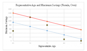
Figure 1: Example of Representative Age and Maximum Savings [1]

each  is shown as brown square. The horizontal axis indicates , while the vertical axis indicates . Regression line  is plotted as dashed blue line in Figure 1.  is shown as Formula (4).

The vertical value obtained through  at each  is defined as predictive value .

Here, the whole set of training data  is defined as “the set whose savings are less than or equal to those of the line  defined as the vertically upward shift of  by the maximum of predicted error at the  of its range focused on” [7]. Predicted error is calculated through subtracting  from . The line  is plotted as solid red line in Figure 1 and expressed as Formula (5).

The maximum of predicted error is 464.5, which is shaded in Table 5. The vertical value obtained through line  at each  is defined as threshold . On top of the maximum ( ), the following three values are also shown in Table 5; predicted value ( ), predicted error ( ), and threshold ( ).

4.2.  Training Data and Partial Sets

Provided that  is the revised disbursement, I is the amount of annual income, and S is the amount of savings, in order to determine the partial sets of training data, the subsequent two conditions are set [7].

1. Revised disbursement is 1.2 times or more than income. ( )
2. Saving is 0.1 times or less than income. ( )

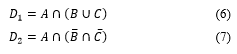
These coefficients, 1.2 and 0.1, are determined through trial and error. As defined in Section 4.1, the training data  is the set that satisfies the amounts of savings are not more than  at . Among the training data , the set that meets the condition 1 (2, respectively) is denoted as  ( ). The partial sets ,  of the training data are then defined as Formulas (6) and (7) [7].

4.3.  Two-Step Methods to Determine Dissaving Risk

The data divided into test data in Section 3.3-(2) is used as test data, while the training data classified in Section 3.3-(2) are used as training data in the following two-step methods. According to the value of  set in the fashion explained in Section 4.1, the dissaving risk against each test data is evaluated through either (1) primary determination or (2) secondary determination stated as follows:

(1) Primary Determination

The data whose savings are not less than  are determined as “no dissaving risk.” The results of primary determination are shown in Table 6. Each column is explained as follows:

• “ ” provides either “ ” or “ .” As stated in Section 3.3-(2), the threshold to determine dissaving risk was set to 0.1 (0.3, respectively) for single males and females (Twos) in the previous analysis [7]. The abbreviation “Act” listed in the second row stands for “Actual,” indicating that  is an actual value.
• “Det” stands for determination. This column provides the result of determining dissaving risk, either “Dissaving Risk” or “No Dissaving Risk.” For Table 6, mere “No Dissaving Risk” is provided, as explained above.
• “T/F” provides whether determination result is correct or not. If the determination result is correct, this column provides “TRUE,” otherwise “FALSE.”
• “Result” is classified as two results in Table 6. The results are “Leak Detection 1 (LD1)” and “No Risk 1 (NR1).”
• “Abb” indicates the abbreviations of results as stated above.
• “Data” indicates the amounts of the data.

Table 6: Primary Determination Results

No.	P	Primary Determination Results
	Act	Det	T/F	Result	Abb	Data
1		No Dissaving Risk	FALSE	Leak Detection 1	LD1
2			TRUE	No Risk 1	NR1

 (2) Secondary Determination

 Secondary determination proceeds through each of three methods, against the test data that have not been determined in primary determination yet.

 (i) Method 1

     For a test data, estimated saving exhaustion term (ESET) is calculated as follows. Provided that  is the revised disbursement, I is the amount of annual income, and S is the amount of savings, similar as Formula (2), ESET can be calculated as using Formula (8).

A further procedure of method 1 will be explained using Figure 2-(a). Here, three training data whose Euclidean distances to the test data are the first to third shortest in terms of savings are extracted from training data belonging to . The criterion of the training data with first to third shortest  determined through trial and error. Among the ESETs of the three training data extracted, the shortest one is set as . In Figure 2-(a), the training data with the shortest is described as a red circle, while the other two are shown as orange circles. The red arrow is then derived from the red circle to a blue circle, the test data, to set the shortest ESET as .

The  of the test data will then be divided by the life expectancy  corresponding to the age group and the year (1994, 1999 or 2004) of the training data. Provided that  is the ratio of  to  for each data, similar as Formula (3),  is calculated through Formula (9).

If  is less than , the threshold to determine dissaving risk, the test data is determined as having “Dissaving risk.” Otherwise as “No dissaving risk.” The results of secondary determination are summarized in Table 7. The columns are basically the same as explained in Section 4.3-(1). Minor differences from Table 6 are explained as follows:

• In the column entitled “ ”, the abbreviation “Est” is listed, indicating that is an estimated value.
• “T/F” provides “TRUE” if the column entitled “Estimated” and “Actual” correspond, otherwise “FALSE.”
• “Result” is classified as four categories in Table 7. The categories are expressed as “Correct Detection (CD),” “Incorrect Detection (ID),” “Leak Detection 2 (LD2)” and “No Risk 2 (NR2).

(ii) Method 2

     For a test data, three training data whose Euclidean distances to the test data are the first to third shortest in terms of savings are extracted from training data belonging to  or . If training data belonging to  account for at least two out of those three, the test data is determined as having “no dissaving risk.” On the other hand, if training data belonging to   account for at least two out of those three, then similar as method 1, three training data whose Euclidean distances to the test data are the first to third shortest in terms of savings are extracted from the training data belonging to . The procedure of method 2 is described in Figure 2-(b), with the case when two training data belonging to . Similar to method 1 and Figure 2-(a), among the training data belonging to , the smallest is set as . Then the test data is determined as having “dissaving risk” if  is less than .

(iii) Method 3

For a test data, three training data whose Euclidean distances to the test data are the first to third shortest in terms of the two-dimensional vector space composed of income and savings are extracted from the training data belonging to  or . Similar to method 2, if training data belonging to  account for at least two out of those three, the test data is determined as having “no dissaving risk.” Meanwhile, if training data belonging to   account for at least two out of those three,  is then obtained as explained in methods 1 and 2. The procedure of method 3 is described in Figure 2-(b). Then the test data are determined as having “dissaving risk” if  is less than .

4.4.  Measures for Performance Evaluation

The data determined as the total six types of the results are summarized in Tables 6 and 7. For convenience, LD1 and LD2 (NR1 and NR2, respectively) are collectively named as LD (NR). Here, correct detection rate (CDR), leak detection rate (LDR) and correct judgment rate (CJR) are calculated as follows.

• CDR means the ratio of the amount of CD to the sum of the data determined as having dissaving risk in the secondary determination. For the denominator, these data are determined as having “Dissaving Risk” in the column entitled “Det” in Table 7 corresponding to the sum of the amount of CD and that of ID. CDR is calculated with Formula (10):

Table 7: Secondary Determination Results

No.			Secondary Determination Results
	Est	Act	Det	T/F	Result	Abb	Data
1			Dissaving Risk	TRUE	Correct Detection	CD
2				FALSE	Incorrect Detection	ID
3			No Dissaving Risk	FALSE	Leak Detection 2	LD2
4				TRUE	No Risk 2	RD2

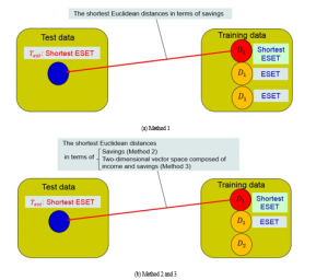
Figure 2: The Procedures of Three Methods for Secondary Determination

• LDR means the ratio of the amount of LD among the data actually determined as having dissaving risk. For the denominator, these data are expressed as “ ” in the column entitled “ ” and “Act” in Tables 6 and 7 corresponding to the sum of the amount of CD and that of LD.  is calculated with Formula (11):

• CJR means the ratio of the sum of amount of CD and the amount of NR to the number of all the analysis data. For the numerator, these data are expressed as “TRUE” in the column entitled “T/F” in Tables 6 and 7. CJR is calculated with Formula (12):

5. Evaluation of Proposed Method through Random Data (RD)

5.1.  Division of Anonymous Data (AD)

The use of AD could be controversial in terms of the safety of its anonymity. In order to enforce the anonymity of AD, random data (RD) is generated along with the AD. For the purpose of performance evaluation, RD is then compared with the case of analyzing mere AD as it is.

Determination method is performed by setting each AD as test data and RD as training data. As a preparation of generating RD, AD (single: 171 males, 1,203 females, Twos: 2,367 households) is divided through the following procedures regarding savings and revised disbursements.

(a) The analysis data is just divided into three datasets according to the amount of saving; high-savings (H-s), medium-savings (M-s), and low-savings (L-s). The thresholds between the datasets are determined as follows:

• In AD, the amount of maximum savings is provided with 5.5 million yen. The threshold between M-s and H-s is set as the average of 0 yen and 5.5 million yen: 2.75 million yen.
• Similarly, the threshold between L-s and M-s is set as the average of 0 yen and 2.75 million yen: 1.375 million yen.

(b) Each of the three datasets divided in (a) is respectively divided into two datasets; high-disbursement (H-d), medium- disbursement (M-d), and low-disbursement (L-d) in accordance with the amount of revised disbursement. The threshold  is set as double of the average of respective datasets. From this viewpoint, for example of single females with own houses,  for L-s (M-s and H-s, respectively) is set as 483.7 (718.4 and 926.7). These dividing methods are determined thorough trial and error. The amounts of analysis data through the procedure are shown in Table 8. Nevertheless, there could be the case where it would be impossible to divide the test data into any smaller groups. Such cases result from insufficient amount of data after they are divided in accordance with savings and revised disbursements. Taking an example of the single males with rent house, there are only nine data whose savings are over 1.375 million yen (M-s and H-s). In such cases, these groups are not divided into smaller ones.

5.2.  Generation of Random Data (RD)

For the analysis data divided into the six attribute datasets as stated in Section 3.3-(3), in accordance with respective savings and revised disbursement, RD are generated along with the following three variables; income, revised disbursement, and savings. Through mvnrnd function implemented in MatLAB [18],  sets ( ) of preliminary RD is generated for each of the respective subdivided datasets in order to avoid failing to extract five sets of RD (amount of data: ) owing to the shortage of preliminary RD.

Table 8: The Amounts of Datasets Divided in Accordance with Saving and Revised Disbursement [1]

(a) Male, Rent                 (b) Male, Own

S\D	L-d	H-d	Total		S\D	L-d	H-d	Total
L-s	52				L-s	58	5	63
M-s	9				M-s	26
H-s					H-s	18	3	21
Total			61		Total			110

(c) Female, Rent            (d) Female, Own

S\D	L-d	H-d	Total		S\D	L-d	H-d	Total
L-s	269	10	279		L-s	529	43	572
M-s	37				M-s	171	9	180
H-s	15				H-s	110	10	120
Total			331		Total			872

(e) Twos, Rent               (f) Twos, Own

S\D	L-d	H-d	Total		S\D	L-d	H-d	Total
L-s	255	10	265		L-s	1388	48	1436
M-s	32				M-s	373	46	419
H-s	5	4	9		H-s	172	34	206
Total			306		Total			2061

Given that income is , revised disbursement is  and amount of savings is , negative values can be automatically and randomly generated for ,  and . Therefore, the data that absolutely meets  are sequentially extracted from the preliminary RD generated through mvnrnd function [18]. Here, the five sets of RD extracted through these procedures for the respective divided datasets are defined as candidate RD.

Next, one of the five sets of the candidate RD must be chosen to use for the subsequent analysis. In terms of savings exhaustion term (SET),  for five sets of RD are compared with  for AD by plotting them. Through visual judgment, one set of RD is chosen whose outline is the most similar to AD. How to determine RD out of the five candidate RD are explained by using the actual example of datasets for female with own house divided into L-s and L-D. SET (  for AD and  for candidate RD) are shown in Figure 3. Here,  and   shown in Figure 3 range from 0 to 30 years. If these terms are beyond 30 years,  or  for those data are regarded as just 30 years. Among these values,  for AD is

Figure 3: Distribution of Saving Exhaustion Term (Female, Own, L-s and L-d)

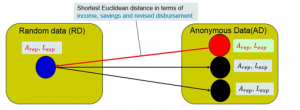
Figure 4: The Procedure of Setting Age Group and Life Expectancy on Random Data (RD) obtained from Anonymous Data (AD)

depicted in Figure 3-(a), while (b)  for the selected RD is shown in Figure 3-(b). On the other hand,  for the candidate RD that are not selected for the subsequent analysis are shown in Figure 3-(c). These candidate RD are named as RD-Cand1, Rd-Cand2, Rd-Cand3 and Rd-Cand4, respectively. Comparing these values, (b)RD resembles (a)AD more than (c)the rest of candidate RD do. Through these procedures, the selected RD for each of the six attribute datasets is utilized for the following analysis.

5.3.  Setting Age Group and Life Expectancy to RD

RD generated and chosen through the procedures described in Section 5.2 already have three attributes; income , revised disbursement  and savings . Nevertheless, age group  and life expectancy  of RD have not been assigned yet. Therefore, it would be necessary to determine these attributes. Here, in the three-dimensional space composed of , for one RD, one among the AD is extracted whose Euclidean distance is shortest. The age group and life expectancy of the AD are then assigned to the RD. The outline of this procedure is shown in Figure 4, similar as that of secondary determination explained in Section 4.3-(2) and shown in Figure 2. One AD with shortest Euclidean distance is denoted as red circle. Then a red arrow starts from the red circle to a blue circle (RD) to set  and . The amounts of AD and those of RD determined through this procedure are shown in Table 9. The column entitled “AD (Test)” indicates the amount of AD data used as test data, whereas the column entitled “RD (Train)” means that of RD used as training data.

Table 9: Amounts of AD and RD [1]

(a) Male, Rent                        (b) Male, Own

Age Group	AD (Test)	RD (Train)		Age Group	AD (Test)	RD (Train)
65 – 69	22	24		65 – 69	37	29
70 – 74	20	20		70 – 74	26	38
75 – 79	11	6		75 – 79	32	31
80 – 84	6	9		80 – 84	10	9
85 –	2	2		85 –	5	3

 (c) Female, Rent        (d) Female, Own

Age Group	AD (Test)	RD (Train)		Age Group	AD (Test)	RD (Train)
65 – 69	101	84		65 – 69	312	324
70 – 74	119	121		70 – 74	286	304
75 – 79	72	100		75 – 79	172	153
80 – 84	29	20		80 – 84	84	78
85 –	10	6		85 –	18	13

 (e) Twos, Rent            (f) Twos, Own

Age Group	AD (Test)	RD (Train)		Age Group	AD (Test)	RD (Train)
65 – 69	154	146		65 – 69	1077	1129
70 – 74	104	114		70 – 74	673	645
75 – 79	38	40		75 – 79	240	227
80 – 84	9	5		80 – 84	67	51
85 –	1	1		85 –	4	9

5.4.  Analysis Results

The validity of AD used along with RD as training data is analyzed in the similar fashion as explained in Section 4.4. Here, RD generated through the method described in Sections 5.1 and 5.2 is utilized as training data, while AD is used as test data. The amounts of partial sets of ,  are shown in Table 10.

There are two slight differences from the previous analysis explained in Section 4.4. Firstly, the threshold  is determined in a subtle different fashion. Similar to the AD, there are several RD with substantially high savings in spite of being determined as dissaving risk. Unlike AD, however, RD have no attributions of consumption items. Here, the distributions of savings for each age group are investigated and plotted. Then higher savings that apparently seem isolated from the other lower ones are then discarded for setting . The thresholds determined are shown in Table 11. Another modification is the threshold  to determinate dissaving risk for single males and females. In the previous analysis, as stated in Section 3.3-(2), the value of  was set to 0.1 for single-person households, as explained in Section 3.3-(2). In this analysis, through trial and error, the threshold is set to 0.15 for single households.

Table 10: Amounts of Partial Sets of D₁ and D₂ [1]

(a) Male, Rent               (b) Male, Own

Age Group	Partial Sets				Age Group	Partial Sets
			Total					Total
65 – 69	5	0	5		65 – 69	13	3	16
70 – 74	3	1	4		70 – 74	17	0	17
75 – 79	1	0	1		75 – 79	13	2	15
80 – 84	0	0	0		80 – 84	5	1	6
85 –	0	0	0		85 –	2	0	2

(c) Female, Rent          (d) Female, Own

Age Group	Partial Sets				Age Group		Partial Sets
			Total						Total
65 – 69	56	12	68		65 – 69		152	33	185
70 – 74	49	20	69		70 – 74		147	33	180
75 – 79	34	4	38		75 – 79		74	14	88
80 – 84	9	2	11		80 – 84		34	8	42
85 –	2	0	2			85 –	8	1	9

(e) Twos, Rent             (f) Twos, Own

Age Group	Partial Sets				Age Group	Partial Sets
			Total					Total
65 – 69	88	39	127		65 – 69	824	212	1036
70 – 74	60	18	78		70 – 74	454	119	573
75 – 79	14	5	19		75 – 79	124	30	154
80 – 84	0	0	0		80 – 84	25	4	29
85 –	1	0	1		85 –	2	0	2

In order to compare the analysis results for this section with the previous ones [7], both of the analysis results are summarized in Tables 12 and 13, respectively. See Appendix on the detailed analysis results; the amounts of data determined as LD1, NR1, CD, ID, LD2 and NR2, and the detailed results for each age group.

In order to compare the differences of results between the analysis using RD (Table 12) and that utilizing mere AD (Table 13), their differences are summarized in Table 14. Here, these values are calculated by subtracting those with AD from those with RD. For CDR and CJR, the bigger they are, the better the result is. Therefore, if these values are positive, they are colored blue. Otherwise, if the values are negative, they are colored red.

For LDR, meanwhile, the smaller it is, the better the result is. Thus, on the contrary to CDR and CJR, if these values are negative, they are colored blue. Otherwise, if the values are positive, they are colored red.

Table 11: Threshold for Analysis Using RD [1]

(a) Male, Rent                               (b) Male, Own

Age Group	Savings				Age Group	Savings
65 – 69	200.0	168.7	200.0		65 – 69	423.8	547.3	978.9
70 – 74	98.6	161.0	192.2		70 – 74	991.3	559.7	991.3
75 – 79	184.5	153.3	184.5		75 – 79	79.8	572.2	1003.7
80 – 84			184.5		80 – 84	769.0	584.6	1016.1
85 –			184.5		85 –			1028.6

(c) Female, Rent                          (d) Female, Own

Age Group	Savings				Age Group	Savings
65 – 69	491.3	593.6	749.7		65 – 69	1034.2	1056.7	1184.5
70 – 74	563.0	487.7	643.8		70 – 74	1052.0	924.2	1052.0
75 – 79	537.9	381.8	537.9		75 – 79	603.3	791.7	919.4
80 – 84	146.6	275.9	432.0		80 – 84	742.0	659.1	786.9
85 –			432.0		85 –			786.9

        (e) Twos, Rent                             (f) Twos, Own

Age Group	Savings				Age Group	Savings
65 – 69	1647.8	1414.0	1647.8		65 – 69	4757.9	4923.1	5236.3
70 – 74	951.4	1040.7	1274.4		70 – 74	3988.0	3674.8	3988.0
75 – 79	333.5	667.3	901.1		75 – 79	2578.8	2426.5	2739.7
80 – 84			527.8		80 – 84	593.1	1178.2	1491.4
85 –	109.9	-79.3	154.5		85 –	213.8	-70.1	243.1

Table 12: Analysis Results with RD [1]

(a) Rent

Methods [%]	Single						Two-person Household
	Male			Female
	CDR	LDR	CJR	CDR	LDR	CJR	CDR	LDR	CJR
Method 1	60.0	0.0	83.6	46.1	11.9	76.7	41.4	16.7	68.3
Method 2	60.0	0.0	83.6	47.2	11.9	77.6	38.3	43.1	68.3
Method 3	65.2	0.0	86.9	47.2	11.9	77.6	38.2	41.7	68.0

(b) Own

Methods [%]	Single						Two-person Household
	Male			Female
	CDR	LDR	CJR	CDR	LDR	CJR	CDR	LDR	CJR
Method 1	57.1	36.8	85.5	38.2	30.3	80.5	31.8	21.1	63.8
Method 2	57.1	36.8	85.5	39.1	35.3	81.4	32.3	29.0	66.0
Method 3	60.0	36.8	86.4	42.4	31.9	83.0	36.0	26.2	70.0

Table 13: Analysis Results with only AD [7]

(a) Rent

Methods [%]	Single						Two-person Household
	Male			Female
	CDR	LDR	CJR	CDR	LDR	CJR	CDR	LDR	CJR
Method 1	100.0	60.0	90.0	56.1	8.0	87.8	32.1	12.9	59.9
Method 2	100.0	60.0	90.0	60.6	20.0	89.0	39.5	50.0	71.7
Method 3	100.0	60.0	90.0	60.0	16.0	89.0	33.3	58.8	68.4

(b) Own

Methods [%]	Single						Two-person Household
	Male			Female
	CDR	LDR	CJR	CDR	LDR	CJR	CDR	LDR	CJR
Method 1	62.5	0.0	94.4	30.4	22.2	83.5	36.5	25.9	68.1
Method 2	50.0	40.0	90.7	32.4	38.9	86.2	36.2	47.7	70.4
Method 3	50.0	40.0	90.7	38.6	38.9	88.8	37.3	49.5	71.5

Table 14: Differences of Results between RD (Table 12) and only AD (Table 13)

(a) Rent

Methods [%]	Single						Two-person Household
	Male			Female
	CDR	LDR	CJR	CDR	LDR	CJR	CDR	LDR	CJR
Method 1	-40.0	-60.0	-6.4	-10.0	3.9	-11.1	9.3	3.8	8.4
Method 2	-40.0	-60.0	-6.4	-13.4	-8.1	-11.4	-1.2	-6.9	-3.4
Method 3	-34.8	-60.0	-3.1	-12.8	-4.1	-11.4	4.9	-17.1	-0.4

(b) Own

Methods [%]	Single						Two-person Household
	Male			Female
	CDR	LDR	CJR	CDR	LDR	CJR	CDR	LDR	CJR
Method 1	-5.4	36.8	-8.9	7.8	8.1	-3.0	-4.7	-4.8	-4.3
Method 2	7.1	-3.2	-5.2	6.7	-3.6	-4.8	-3.9	-18.7	-4.4
Method 3	10.0	-3.2	-4.3	3.8	-7.0	-5.8	-1.3	-23.3	-1.5

From the viewpoints of CDR and CJR, for the data with rent house, deterioration is observed in most cases except some for Twos: CDR and CJR for method 1, and CDR for method 3. For the data with own house, CDR is improved for single households except for males for method 1, while it becomes degraded for Twos. CJR becomes deteriorated for both single-person and two-person households. On the other hand, LDR is improved for most of the cases except those with method 1 for Twos with rent and males with own.

5.5.  Considerations

Comparing the three methods using RD (Table 12), from the viewpoints of CDR and CJR, as a whole, CDR and CJR become best with method 3. However, for the data with rent house, CDR and CJR equally show similar performance for methods 2 and 3. For Twos, method 1 outperforms the others. From the viewpoint of LDR, on the other hand, method 1 works best since LDR is the lowest value among the three methods for all the cases. Therefore,  method 3 is best in light of CDR and CJR, whereas there is room for improvement for LDR. Meanwhile, method 1 is better than the others considering LDR, while it leaves much to be desired for CDR and CJR.

In the light of the differences of analysis results between RD and AD (Table 14), as a whole, LDR is improved, while CDR and CJR are deteriorated. However, these analysis results are dependent on RD and can be variable. As limitations of analysis, AD are required to be returned within the designated periods [8]. Moreover, there could be insufficient analysis data with certain attributes, especially males. How to cope with the situation where there is not enough data is our requirement for the further analysis.

Nevertheless, these two types of analysis results show the similar results for all the three methods. Therefore, it could be concluded that using RD along with the AD for evaluating the performance of the proposed method [7] could be effective.

6. Conclusion

In the reported study [7], we proposed a method to detect dissaving risk of people at the age of sixty-five or older for AD. In order to strengthen the anonymity of the data, RD used along with the AD is generated and then compared with the previous analysis, with a view to performance evaluation [1]. Here, AD is set as test data, whereas RD is used as training data. As a result of analysis, from the viewpoints of CDR and CJR, for the data with rent house, degradation was observed with most cases. On the other hand, for the data with own house, CDR was improved with most cases for single-person households, while it became deteriorated for Twos. CJR dropped for both single-person and two-person households. Meanwhile, LDR was improved for most of the cases. As a whole, it could be concluded that using RD might be as effective as using AD for evaluating the performance of the proposed method [7].

For future work, while CJR exceeded 80% for single-person households, it attained as high as approximately 70% for two-person households. Therefore, CDR and CJR especially for the data of two-person households must be improved. How to deal with the cases with insufficient analysis data for further analysis is included in our future works.

Acknowledgment

This research was supported by the Research Institute of Science and Technology for Society within the Japan Science and Technology Agency.

Appendix

The detailed analysis results of Table 12 for rent for males, own for males, rent for females, own for females, rent for Twos, and own for Twos are shown in Table A.1 (a), (b), (c), A.2 (a), (b), (c), A.3 (a), (b), (c), A.4 (a), (b), (c) , A.5 (a), (b), (c) , and A.6 (a), (b), (c), respectively.

Table A.1 (a): The Detailed Analysis Results (Male, Rent: Method 1)

Age Group	Preliminary			Secondary					T	Results
	LD1	NR1	T	CD	ID	LD2	NR2	T		CDR	LDR	CJR
65-69	0	15	15	5	2	0	0	7	22	71.4	0.0	90.9
70-74	0	13	13	3	4	0	0	7	20	42.9	0.0	80.0
75-79	0	3	3	6	2	0	0	8	11	75.0	0.0	81.8
80-84	0	3	3	1	2	0	0	3	6	33.3	0.0	66.7
85-	0	1	1	0	0	0	1	1	2	–	–	100.0
T	0	35	35	15	10	0	1	26	61	60.0	0.0	83.6

Table A.1 (b): The Detailed Analysis Results (Male, Rent: Method 2)

Age Group	Preliminary			Secondary					T	Results
	LD1	NR1	T	CD	ID	LD2	NR2	T		CDR	LDR	CJR
65-69	0	15	15	5	2	0	0	7	22	71.4	0.0	90.9
70-74	0	13	13	3	4	0	0	7	20	42.9	0.0	80.0
75-79	0	3	3	6	2	0	0	8	11	75.0	0.0	81.8
80-84	0	3	3	1	2	0	0	3	6	33.3	0.0	66.7
85-	0	1	1	0	0	0	1	1	2	–	–	100.0
T	0	35	35	15	10	0	1	26	61	60.0	0.0	83.6

Table A.1 (c): The Detailed Analysis Results (Male, Rent: Method 3)

Age Group	Preliminary			Secondary					T	Results
	LD1	NR1	T	CD	ID	LD2	NR2	T		CDR	LDR	CJR
65-69	0	15	15	5	2	0	0	7	22	71.4	0.0	90.9
70-74	0	13	13	3	3	0	1	7	20	50.0	0.0	85.0
75-79	0	3	3	6	1	0	1	8	11	85.7	0.0	90.9
80-84	0	3	3	1	2	0	0	3	6	33.3	0.0	66.7
85-	0	1	1	0	0	0	1	1	2	–	–	100.0
T	0	35	35	15	8	0	3	26	61	65.2	0.0	86.9

Table A.2 (a): The Detailed Analysis Results (Male, Own: Method 1)

Age Group	Preliminary			Secondary					T	Results
	LD1	NR1	T	CD	ID	LD2	NR2	T		CDR	LDR	CJR
65-69	2	24	26	5	3	0	3	11	37	62.5	28.6	86.5
70-74	3	12	15	5	3	1	2	11	26	62.5	44.4	73.1
75-79	0	26	26	1	2	0	3	6	32	33.3	0.0	93.8
80-84	1	7	8	1	1	0	0	2	10	50.0	50.0	80.0
85-	0	3	3	0	0	0	2	2	5	–	–	100.0
T	6	72	78	12	9	1	10	32	110	57.1	36.8	85.5

Table A.2 (b): The Detailed Analysis Results (Male, Own: Method 2)

Age Group	Preliminary			Secondary					T	Results
	LD1	NR1	T	CD	ID	LD2	NR2	T		CDR	LDR	CJR
65-69	2	24	26	5	3	0	3	11	37	62.5	28.6	86.5
70-74	3	12	15	5	3	1	2	11	26	62.5	44.4	73.1
75-79	0	26	26	1	2	0	3	6	32	33.3	0.0	93.8
80-84	1	7	8	1	1	0	0	2	10	50.0	50.0	80.0
85-	0	3	3	0	0	0	2	2	5	–	–	100.0
T	6	72	78	12	9	1	10	32	110	57.1	36.8	85.5

Table A.2 (c): The Detailed Analysis Results (Male, Own: Method 3)

Age Group	Preliminary			Secondary					T	Results
	LD1	NR1	T	CD	ID	LD2	NR2	T		CDR	LDR	CJR
65-69	2	24	26	5	3	0	3	11	37	62.5	28.6	86.5
70-74	3	12	15	5	3	1	2	11	26	62.5	44.4	73.1
75-79	0	26	26	1	1	0	4	6	32	50.0	0.0	96.9
80-84	1	7	8	1	1	0	0	2	10	50.0	50.0	80.0
85-	0	3	3	0	0	0	2	2	5	–	–	100.0
T	6	72	78	12	8	1	11	32	110	60.0	36.8	86.4

Table A.3 (a): The Detailed Analysis Results (Female, Rent: Method 1)

Age Group	Preliminary			Secondary					T	Results
	LD1	NR1	T	CD	ID	LD2	NR2	T		CDR	LDR	CJR
65-69	1	31	32	20	19	1	29	69	101	51.3	9.1	79.2
70-74	2	50	52	26	23	3	15	67	119	53.1	16.1	76.5
75-79	0	35	35	10	14	1	12	37	72	41.7	9.1	79.2
80-84	0	15	15	2	12	0	0	14	29	14.3	0.0	58.6
85-	0	6	6	1	1	0	2	4	10	50.0	0.0	90.0
T	3	137	140	59	69	5	58	191	331	46.1	11.9	76.7

Table A.3 (b): The Detailed Analysis Results (Female, Rent: Method 2)

Age Group	Preliminary			Secondary					T	Results
	LD1	NR1	T	CD	ID	LD2	NR2	T		CDR	LDR	CJR
65-69	1	31	32	20	16	1	32	69	101	55.6	9.1	82.2
70-74	2	50	52	26	23	3	15	67	119	53.1	16.1	76.5
75-79	0	35	35	10	14	1	12	37	72	41.7	9.1	79.2
80-84	0	15	15	2	12	0	0	14	29	14.3	0.0	58.6
85-	0	6	6	1	1	0	2	4	10	50.0	0.0	90.0
T	3	137	140	59	66	5	61	191	331	47.2	11.9	77.6

Table A.3 (c): The Detailed Analysis Results (Female, Rent: Method 3)

Age Group	Preliminary			Secondary					T	Results
	LD1	NR1	T	CD	ID	LD2	NR2	T		CDR	LDR	CJR
65-69	1	31	32	20	16	1	32	69	101	55.6	9.1	82.2
70-74	2	50	52	26	23	3	15	67	119	53.1	16.1	76.5
75-79	0	35	35	10	14	1	12	37	72	41.7	9.1	79.2
80-84	0	15	15	2	11	0	1	14	29	15.4	0.0	62.1
85-	0	6	6	1	2	0	1	4	10	33.3	0.0	80.0
T	3	137	140	59	66	5	61	191	331	47.2	11.9	77.6

Table A.4 (a): The Detailed Analysis Results (Female, Own: Method 1)

Age Group	Preliminary			Secondary					T	Results
	LD1	NR1	T	CD	ID	LD2	NR2	T		CDR	LDR	CJR
65-69	4	148	152	37	45	11	67	160	312	45.1	28.8	80.8
70-74	5	127	132	26	48	9	71	154	286	35.1	35.0	78.3
75-79	1	77	78	12	22	3	57	94	172	35.3	25.0	84.9
80-84	0	40	40	8	19	1	16	44	84	29.6	11.1	76.2
85-	0	7	7	0	0	2	9	11	18	–	100.0	88.9
T	10	399	409	83	134	26	220	463	872	38.2	30.3	80.5

Table A.4 (b): The Detailed Analysis Results (Female, Own: Method 2)

Age Group	Preliminary			Secondary					T	Results
	LD1	NR1	T	CD	ID	LD2	NR2	T		CDR	LDR	CJR
65-69	4	148	152	36	41	12	71	160	312	46.8	30.8	81.7
70-74	5	127	132	24	47	11	72	154	286	33.8	40.0	78.0
75-79	1	77	78	11	16	4	63	94	172	40.7	31.3	87.8
80-84	0	40	40	6	16	3	19	44	84	27.3	33.3	77.4
85-	0	7	7	0	0	2	9	11	18	–	100.0	88.9
T	10	399	409	77	120	32	234	463	872	39.1	35.3	81.4

Table A.4 (c): The Detailed Analysis Results (Female, Own: Method 3)

Age Group	Preliminary			Secondary					T	Results
	LD1	NR1	T	CD	ID	LD2	NR2	T		CDR	LDR	CJR
65-69	4	148	152	39	38	9	74	160	312	50.6	25.0	83.7
70-74	5	127	132	24	47	11	72	154	286	33.8	40.0	78.0
75-79	1	77	78	12	15	3	64	94	172	44.4	25.0	89.0
80-84	0	40	40	6	10	3	25	44	84	37.5	33.3	84.5
85-	0	7	7	0	0	2	9	11	18	–	100.0	88.9
T	10	399	409	81	110	28	244	463	872	42.4	31.9	83.0

Table A.5 (a): The Detailed Analysis Results (Twos, Rent: Method 1)

Age Group	Preliminary			Secondary					T	Results
	LD1	NR1	T	CD	ID	LD2	NR2	T		CDR	LDR	CJR
65-69	4	35	39	34	43	4	34	115	154	44.2	19.0	66.9
70-74	1	34	35	23	31	2	13	69	104	42.6	11.5	67.3
75-79	1	18	19	3	9	0	7	19	38	25.0	25.0	73.7
80-84	0	6	6	0	2	0	1	3	9	0.0	–	77.8
85-	0	1	1	0	0	0	0	0	1	–	–	100.0
T	6	94	100	60	85	6	55	206	306	41.4	16.7	68.3

Table A.5 (b): The Detailed Analysis Results (Twos, Rent: Method 2)

Age Group	Preliminary			Secondary					T	Results
	LD1	NR1	T	CD	ID	LD2	NR2	T		CDR	LDR	CJR
65-69	4	35	39	25	31	13	46	115	154	44.6	40.5	68.8
70-74	1	34	35	14	25	11	19	69	104	35.9	46.2	64.4
75-79	1	18	19	2	8	1	8	19	38	20.0	50.0	73.7
80-84	0	6	6	0	2	0	1	3	9	0.0	–	77.8
85-	0	1	1	0	0	0	0	0	1	–	–	100.0
T	6	94	100	41	66	25	74	206	306	38.3	43.1	68.3

Table A.5 (c): The Detailed Analysis Results (Twos, Rent: Method 3)

Age Group	Preliminary			Secondary					T	Results
	LD1	NR1	T	CD	ID	LD2	NR2	T		CDR	LDR	CJR
65-69	4	35	39	23	37	15	40	115	154	38.3	45.2	63.6
70-74	1	34	35	16	24	9	20	69	104	40.0	38.5	67.3
75-79	1	18	19	3	6	0	10	19	38	33.3	25.0	81.6
80-84	0	6	6	0	1	0	2	3	9	0.0	–	88.9
85-	0	1	1	0	0	0	0	0	1	–	–	100.0
T	6	94	100	42	68	24	72	206	306	38.2	41.7	68.0

Table A.6 (a): The Detailed Analysis Results (Twos, Own: Method 1)

Age Group	Preliminary			Secondary					T	Results
	LD1	NR1	T	CD	ID	LD2	NR2	T		CDR	LDR	CJR
65-69	4	98	102	190	392	47	346	975	1077	32.6	21.2	58.9
70-74	1	111	112	98	194	23	246	561	673	33.6	19.7	67.6
75-79	1	74	75	19	69	5	72	165	240	21.6	24.0	68.8
80-84	0	43	43	3	9	1	11	24	67	25.0	25.0	85.1
85-	1	3	4	0	0	0	0	0	4	–	100.0	75.0
T	7	329	336	310	664	76	675	1725	2061	31.8	21.1	63.8

Table A.6 (b): The Detailed Analysis Results (Twos, Own: Method 2)

Age Group	Preliminary			Secondary					T	Results
	LD1	NR1	T	CD	ID	LD2	NR2	T		CDR	LDR	CJR
65-69	4	98	102	171	334	66	404	975	1077	33.9	29.0	62.5
70-74	1	111	112	95	186	26	254	561	673	33.8	22.1	68.4
75-79	1	74	75	10	57	14	84	165	240	14.9	60.0	70.0
80-84	0	43	43	3	9	1	11	24	67	25.0	25.0	85.1
85-	1	3	4	0	0	0	0	0	4	–	100.0	75.0
T	7	329	336	279	586	107	753	1725	2061	32.3	29.0	66.0

Table A.6 (c): The Detailed Analysis Results (Twos, Own: Method 3)

Age Group	Preliminary			Secondary					T	Results
	LD1	NR1	T	CD	ID	LD2	NR2	T		CDR	LDR	CJR
65-69	4	98	102	179	326	58	412	975	1077	35.4	25.7	64.0
70-74	1	111	112	93	136	28	304	561	673	40.6	23.8	75.5
75-79	1	74	75	15	45	9	96	165	240	25.0	40.0	77.1
80-84	0	43	43	3	9	1	11	24	67	25.0	25.0	85.1
85-	1	3	4	0	0	0	0	0	4	–	100.0	75.0
T	7	329	336	290	516	96	823	1725	2061	36.0	26.2	70.0

1.  Y. Yokoyama and Y. Yoshitomi, “Assessment of Dissaving Risk against Life Expectancy for Elderly People through Anonymous Data and Random Data,” Proc. of the 20th ACIS International Conference on Software Engineering, Artificial Intelligence, Networking and Parallel/Distributed Computing (SNPD 2019), 274-279, 2019, doi: 10.1109/SNPD.2019.8935718.
2. H. Ohba, Y. Kadoya, and J. Narumoto, “Influence on the household change Caused by Dementia Decline -Two-year Longitudinal Analysis Using JSTAR Data-” (in Japanese), Proc. of the 20th Japan Society of Geriatric & Gerontological Behavioral Sciences, 2017.
3. Aomori Prefectural Industrial Technology Research Center, etc., “Dementia Prediciton Program and Method” (in Japanese), Japan patent JP2015-138488A, 2015-07-31.
4. Toshiba Corporation, “Dementia Determination Device, Sysyem, Method, and Program” (in Japanese), Japan patent JP2017-104289A, 2017-06-15.
5. e-Stat: Search for statistics (URL): https://www.e-stat.go.jp/en/stat-search/database?page=1, 2021-4-2.
6. Y. Yokoyama and Y. Yoshitomi, “A Method to Assess Dissaving Risk against Life Expectancy for Elderly People,” Proc. of the 20th ACIS International Conference on Software Engineering, Artificial Intelligence, Networking and Parallel/Distributed Computing (SNPD 2019), 262-267, 2019, doi: 10.1109/SNPD.2019.8935809.
7. Y. Yokoyama and Y. Yoshitomi, “A Method to Determine Dissaving Risk of Elderly People” (in Japanese), Abstracts of the 2019 Spring National Conference of Operations Research Society of Japan, 240-241, 2-F-11, 2019.
8. National Science Center: Use of Anonymous Data (URL, in Japanese), https://www.nstac.go.jp/services/anonymity.html, 2021-4-2.
9. T. Fujita, S. Ogano, and J. Narumoto, “Dementia and Information” (in Japanese), ISBN978-4-326-44976-7, Keisou Shobou, 150, 2019.
10. K. L. Triebel, R. Martin, H. R. Griffith, J. Marceaux, O. C. Okonkwo, L. Harrell, D. Clark, J. Brockington, A. Bartolucci and D. C. Marson, “Declining Financial Capacity in Mild Cognitive Impairment: A one-year Longitudinal Study”, Neurology, 73, 928-934, 2009, doi: 10.1212/WNL.0b013e3181b87971
11. D. Bisdee, D. Price and T. Daly, “Coping with Age-related Threats to Role Identity: Older Couples and the Management of Household Money,” Journal of Community & Applied Social Psychology, 23, 505-518, 2013, doi: 10.1002/casp.2149
12. M. S. Finke, J. S. Howe and S. J. Huston, “Old Age and the Decline in Financial Literacy,” Management Science, 63(1), 213-230, 2017, doi: 10.2139/ssrn.1948627
13. J. W. Hsu and R. Willies, “Dementia Risk and Financial Decision Making by Older Households: The Impact of Information,” Journal of Human Capital, 7(4), 340-377, 2013, doi: 10.2139/ssrn.2339225
14. H. Sakurai and T. Moriwaki, “The Effectiveness of the Default Risk Assessment Based on the Financial Ratios” (in Japanese), Journal of Economics & Business Administration, 214(2), 1-17, 2016.
15. T. Izumi, “Analysis on Consumption by Elder Family Type of Household based on the National Survey of Family Income and Expenditure” (in Japanese), Kaetsu University Research Review, 59(2), 55-67, 2016.
16. National Statistic Center (URL), https://www.nstac.go.jp/en/, 2021-4-2.
17. Life expectancies at specified ages (URL), https://www.mhlw.go.jp/english/database/db-hw/lifetb04/1.html, 2021-4-2.
18. MatLAB: mvnrnd (URL), https://jp.mathworks.com/help/stats/mvnrnd.html?lang=en/index.html, 2021-4-2.

(Click Here)