1.Introduction

The Arkansas River is a crucial element in the economy of the state of Colorado, in the western United States. It is a vital transportation channel and main source of water for irrigated agriculture. Water sources for the river mainly from snowmelt.

Snow melt is a critical component of the water cycle in the American West, providing the region with at least 50% of its annual runoff, and up to 80% in some years. Concerns are growing regarding the impacts the altered climate might have on snowpack and the region’s water cycle overall. A few studies projected the region to have profound changes in minimum winter temperatures, summer average temperatures, snowfall, snow-melt, and growing season rainfall quantities [1]-[5]. Several other studies have reported that spring and early summer temperatures are expected to increase while the quantity of snowpack in spring is expected to decrease [6]-[8].  There are other several earlier studies of snowmelt dominated systems show similar seasonal shifts in snowmelt runoff as a result of warmer temperatures and a shorter snow accumulation period [8]-[11].

If the changes in climate take place as projected, it is expected to have profound impacts on the hydrology of the Arkansas River and hence the economy of the region. Many studies, using historical data analyses, have explored the impacts of climate change on water in this region where water is already under stress [12]–[19]. The outcome of these studies reported that, even though, the direction and magnitude of change in climate is well documented (increase in temperature) but there is no consensus on the direction and magnitude of the impacts on the region. And this attributed to uncertainty regarding the changes in precipitation’s patterns under warmer climate. But, precipitation is the main driving factor of the changes in streamflow. Almost all of the studies conducted in this region, have reported that snow is expected to melt early shifting the peak runoff and the growing season to take place earlier. But none of them reported increases in streamflow. However, the changes in precipitation regimes are expected to cause the snowpack to decrease and/or to melt (shift) earlier. Therefore, streamflow is expected to decrease and the peak emanates earlier shifting the growing season towards winter season [6], [13], [16]. Some studies on the region, projected a reduction in streamflow up to 30% below the historical recorded flow [18]. More recent studies using data sets extracted from GCMs support this result projecting a reduction in streamflow ranges between 10 – 30% by the end of the 21st century [6], [13]-[14]. The only increase in streamflow resulted from increase in precipitation was reported by Groisman and others [20].

It is noticeable, from the outcome of all these studies that there is no consensus on the magnitude and direction of the change in the precipitation and hence the river flow under the changing climatic conditions. This may be attributed to the nature of the climate and hydrologic models used (coarse spatial and temporal resolution).  The coarse resolution bounds the general circulation models (GCMs) to reproduce a similarly complex spatial environment that simulates the actual precipitation. Besides, the discrepancies in the precipitation projections are larger than the ones in the temperature projections [21]-[23].

Scale is crucial for climate and hydrologic modeling. It is reported that the signal of climate change on monthly patterns of runoff is stronger than the annual ones [23], [24]. Projections at finer scales is necessary to better evaluate the impacts the changing climate might have on the hydrology in the region [25]. Therefore, in this research, streamflow is linked to climate change scenarios on a monthly scale and aggregated to annual and decadal scale.

Series of climate parameters (scenarios) have been projected to simulate the changes in climate in the future. Most of these scenarios were developed assuming equilibrium (change in climate caused by jumps in CO2 levels in the atmosphere sometime in the future). In fact, climate is expected to have linear trend of change (transient) following the linear trend of CO2 on the earth [26], [27]. Even though, transient scenarios have not been widely used in studies of climate change. As such, it is necessary to explore their impact, as:

• Transient studies provide deeper insight on trends in climatic change and annual variability;
• Transient projections can indicate the potential rate of change, which is crucial in determining how to respond and adapt to that change, and;
• Transient simulations may give a more accurate picture of the likelihood of when certain critical thresholds will be crossed [27].

This research aims to demonstrate how transient scenarios are better able to evaluate the implications the changing climate might have on river flow at scale. These findings can be particularly useful in supporting or facilitating more informed and higher quality decision-making for water planning and management.

2. Description of the Study Area

The subject of this study is the Arkansas River Basin in Colorado which is enclosed by the Rocky Mountains to the west and Kansas to the east and expanding towards New Mexico and Oklahoma to the south. (Figure 1), the surface area of the basin is approximately 72,742 km2 (28,415 square miles) and accounts for about 27% of the land area of the state of Colorado. The river’s headwaters can be found at over 3,050m (10,000 feet) above sea level, in the vicinity of Leadville, CO. From there, its elevation drops rapidly as the river flows out of the mountains near Pueblo, CO and continues eastward towards the border with Kansas border, near the town of Holly, where the elevation drops to roughly 1,036 m (3,400 feet).

The basin sees a wide range of temperatures and precipitation due to variations in topography. The temperature can see average annual lows of about 2^oC at the basin’s highest point in the mountains and can reach average highs of about 12°C in the lower valley. Seasonal variations are also significant, illustrated by the. the average frost free season (0^oC) ranging from a low of 85 days at Leadville to a high of 167 days at Canon City.

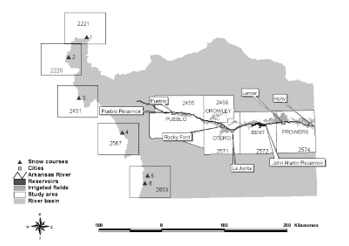Figure 1: Features of the study area in the Arkansas River Basin, Colorado

Precipitation also demonstrates significant variability throughout the year, ranging from 229-305 mm annually in the middle and eastern parts of the basin, to 406-508 mm in the center and east, to a range of 406-508 mm in the west, and as much as 1143 mm at the highest elevations in the mountains. At these heights, much of the precipitation manifests as snow, the runoff of which accounts for the bulk of the region’s annual water supply. Consequently, the size of the water supply is dependent on the volume of winter snowpack and can shift from year to year. However, in general, on average, over 60% of the annual runoff takes place in late spring and mid-summer between April and July, with a further 20% occurring in later summer  and early autumn between August and October [28].

3. Data

The underlying data for this study is in two parts: (1) historical climate scenarios and (2) future climate scenarios. It was sourced from the Vegetation-Ecosystem Modeling and Analysis Project (VEMAP) [29] which collected extensive climate data for the contiguous United States and includes historical data dating back to 1895 and up to 1993, supplemented by projections from two GCM-based scenario models covering the period from 1994-2099.

The historical scenarios were based on data records of varying length from 1,200 stations for the 105-year period between 1895 to 2000 as well as shorter records from approx. 6,000 to 8,000 stations for the 50-year period between 1951 to 2000. Both GCM models, the HAD model and the CCC model, further output climate scenarios with the underlying assumption that carbon dioxide concentrations are progressively increasing at a rate of 1% every year (transient). The VEMAP divided the continental US into a grid with 0.5^o x 0.5^o cells and used these to generate scenarios that would demonstrate the impact of factors such as topography and local ecosystems on climate [29]. The project sponsor, the National Center for Atmospheric Research (NCAR), used a downscaling technique, spatial interpolation to topographically adjust both the historical and projected climate data to fit the small grid cells. The downscaling process took into account the impact of local topography on climate parameters. Figure 2 shows adjusted projections (downscaled) from both models as well as the mean +/- 1 standard deviation for each parameter.

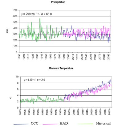Figure 2: Historical and the future scenarios of Precipitation and Temperature

The historical data, sourced from the U.S. Geological Survey (USGS) [30], captures flow levels for the Arkansas River near Pueblo, on a monthly basis between 1900 and 2000. Figure 3 shows the average monthly distribution of the river flow with data collected over 30 years.

As shown in Figure 1, climate data (precipitation & temperature) was collected from five snow courses (grid cells) in the Rocky Mountains a sample which represent overall runoff in the region. Each individual cell contains a minimum of one course upon which runoff forecasts were based. Since the accuracy of the model’s simulations depends heavily on the accuracy of the input data as well as the temporal and spatial scale, the selected snow courses were vetted to ensure accurate and reliable records that reflect the natural runoff and correlated highly snowmelt levels across the entirety of the region [28]. The selected courses, as well as their grid cell number are listed in the adjacent table below (Table 1).

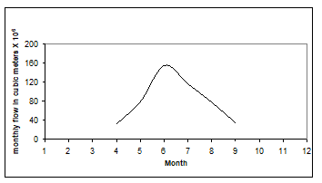Figure 3: Seasonal Cycle of the Arkansas River at Pueblo

Table 1: Characteristics of Snow Courses

Station	Latitude (deg)	Longitude (deg)	Elevation (m)	Cell #
Apishapa	37.33	105.07	3,040	2683
Brumley	39.08	106.53	3,222	2220
Fremont Pass	39.38	106.20	3,465	2221
Prophyry	38.48	106.33	3,271	2451
South Colony	37.97	105.53	3,294	2567
Whiskey Creek	37.22	105.12	3,117	2683

4. Methods

In this paper, in order to study the changes in the river flow that would accompany any climatic changes in the future, we used climate scenarios (precipitation and temperature) extracted from two General Circulation Models (GCM). Namely, the Hadley Centre for Climate Prediction and Research (HAD) and the Canadian Climate Centre (CCC). The data from these two GCMs is of transient nature (gradual change) and high spatial and temporal resolution. To account for spatial variability, the climate data was scaled-down and then used to quantify the impacts the climate change might have on the monthly flows of the river (Arkansas River).  The paper focused to explore the changes in streamflow during the period of April-September, because this is the growing season in the region, and the time during which the effective runoff is usually generated. The monthly flow in the river was simulated using artificial neural network (ANN). The neural network models have been proved to be capable to transform minimum number of inputs into an output [31] – [33]. The neural network model was used for the minimum number of the input data sets it requires. The model was calibrated and validated using 100-years of historical data records. To account for the extrapolation, the historical data was reinforced by extreme events that supposed to resemble the climate conditions under global warming. The ANN model was then used to simulate the river flow under global warming conditions. The output (simulations) from both models (GCM and ANN) are compared to historical records (baseline) to estimate the quantity and extent of the change.

4.1. Modeling Streamflow

The model developed can be described as feedforward artificial neural network (ANN). It is three-layer network; in the middle layer there is a function that map the relationship between the inputs in the first layer (precipitation (PPTa) and temperature (T)) and the outputs in the last layer (streamflow (Qr). The ANN is well formulated in the following form:

Q_r(t) = f(PPTa, T)                        (1)

Here, Qr represents the average monthly streamflow whereas PPTa represents precipitation (accumulated from October of the preceding year, up to each individual month of the year after). To illustrate, the value of PPTa in April would be equal to the cumulative levels of snowpack between October and April. The variable T, meanwhile, represents the average temperature (calculated between April and each individual month in the model). Again, to illustrate, the value of T for May is equal to the average temperature between and April and May. For the month of April itself, we substituted the average March temperature. Accumulating precipitation and temperature was found to contain stronger signals of climate variability. The input data to the ANN was normalized to fall in the range (-1, 1). Normalization is required to remove geometrical biases and equally distribute importance of each input.

4.2. Model Testing and Validation

Data records of 100 years (1900 -2000) were used in training, validating, and testing the neural network. Sixty years of data records 1(900-1960) were used for model’s training, 14 years (1961-1975) were used for validation, and 24 years (1976-2000) were used for testing.

The developed neural network was found favorably capable to simulate the river flow (output) when the precipitation and temperature were used as inputs. The parameters shown in Table 2 summarize the validity of the model. The correlation coefficient (R) is usually used to show the degree of connection between two variables. The values of R range from zero as minimal to one as optimal (0, 1). The Root Mean Square Error (RMSE) is used to determine the magnitude of departure (residual variance) of simulated values from measured ones; the zero value indicates the least magnitude of departure (optimal value).

However, the values of the presented parameters (R and RMSE) document the high correlation between the measured and predicted values and hence the validity of the developed model.

Table 2: Summary of the Model Validation and Testing

Month	Training		Testing
	R	RMSE	R	RMSE
April	0.634	0.17	0.562	0.24
May	0.790	0.10	0.770	0.18
June	0.863	0.11	0.847	0.15
July	0.899	0.06	0.740	0.13
August	0.852	0.06	0.781	0.12
September	0.904	0.07	0.769	0.17

5. Results and Discussion

5.1. Climatic changes

To determine the directionality of the climate change in the region, the main features of the climate scenarios generated from the two GCMs are presented. For better presentation the climate scenarios were aggregated into decadal monthly mean.

Fig. 4 shows the changes in the average monthly temperatures under the two scenarios (HAD and the CCC). The GCMs predicted slight increase in temperature (the region is projected to be warmer). There is a very clear gradual increase in temperature. The change in temperatures during the winter (Dec – Feb) is predicted to be comparatively higher than in the summer (June – August). The changes in temperature look high when compared to the very low historical series of temperatures in winter.

During the focus period (April–September) the temperature average is predicted to increase by 5°C in the 2090s, with a growth rate of 0.45°C every decade. Generally, the 2090s is predicted to be the warmest decade. The figure shows that the CCC scenario predicted higher temperatures in the region compared to the HAD scenario. However, the temperature projections, generated by both scenarios, are similar in trend of change.

Fig. 5 shows the changes in monthly precipitation in decades. It is shown that the HAD scenario predicted large and sudden changes in the average monthly precipitation. Despite the variation, the figure shows a clear pattern in the decadal mean. The figure shows an increase in the decadal mean from the 2010s to 2030s. The increase was gradual at a rate of 1.4% per decade. The 2040s and 2050s noticeably experienced a drop in the decadal mean.  The drop was gradual and rapid at a rate of 1.4% per decade. Then a gradual increase took place again. There was rapid and gradual increase in the decadal mean from 2060s to the 2090s with a growth rate of 2.2% every decade. The projected drop in precipitation could be attributed to changes in natural, large-scale features of the climate: the El Niño Southern Oscillation (ENSO), El Niño, and La Niña [20]-[24].

In general, under the HAD scenario, the increase of the precipitation above the historical base line is expected to be of magnitude of 36% in the spring and of 25% in the summer. On the other hand, it is shown that the CCC scenario predicts a drier

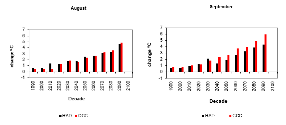Figure 4:  Departures, form historical distribution, of temperature projections from the GCMs:  HAD/CCC

Figure 5:  Departures form historical distribution of precipitation projections from the GCMs:  HAD/CCC

climate for the region. The projections of the CCC show no clear departure from the historical levels except for the 2080s where a the region was projected to have significant increase (9% above the baseline). Worth to mention, the driest climate is expected during the 2040s with a departure of 7%, below the historical levels, in April, 4% in August, and 47% in October.   However, the CCC tends to project precipitation patterns with no clear trend and less variability compared to the HAD. Generally, the two scenarios, show poor similarity in the trend and the extent of change in the precipitation projections.

5.2. Impacts on Streamflow

Figure 6 shows the projections of streamflow. The projections are compared to the historical flow distribution. In spring season, under the HAD scenario, driven by the projected increases in precipitation shown in Figure 5, the results show a large increases in future monthly streamflow. Compared to historical records, the average monthly streamflow increased by 87% for the 2030s and 2050s. The increase jumped to an average of 200% for the 2070s, 2080s, and 2090s. In summer, the increases are projected to be less ranging from 39% for the 2030s to 74% for 2090s. In the fall, dampened by the increase in temperature, the increase in streamflow dropped to 5% in 2030s and to 15 % in 2090s. In general the results show that the largest departures (increases) in flow occur in late spring (April) through early summer (June). This is attributed to the early melting of snow in the mountains. The combined effect of high temperatures and increase in winter snow leads to early snowmelt. However, as a result of change in climate, the peak flow is expected to occur in April rather than June.

The CCC scenario projects a drier climate than the HAD one. Driven by the projected decreases in precipitation shown in Figure 5, the results show that, for 2030s and 2050s, the future monthly streamflow experiences a very slight decrease (5%) in the summer and negligible change in the spring and the fall.  For the 2070s and 2090s, the results show a considerable increase (65%) in the spring and negligible change in the fall. The fluctuations (decreases and increases) in projections of the streamflow are attributed to the annual and decadal variability in the projected changes in climate. The results presented here is widely supported by other several earlier studies conducted on the region [7], [9], [13]-[15].

Figure 7 shows the frequency analysis results of the monthly flow during the focus period (April – September). The results are presented in terms of flow duration curves (FDC). In general, FDC are used to depict the percentage of time the flow in the future exceeds the current levels of flow (historical). Under the CCC scenario the percent of exceedance is almost nil for all months. Under the HAD scenario the percent of exceedance is high for all months (April – September). The flow duration curve falls above the historical (baseline) curve, indicating that the river flow in the future exceeds the current flow value (historical). The probability of exceedance differs from month to month; it is relatively high in the months of April to July and low in August. In September the probability of exceedance almost nil because the two flow curves (historical and future) look similar and almost coincide. The variability in the projected flow is greater in April-July, indicated by the steep flow curves, and stable in August and September inferred by the gentle flow curves.

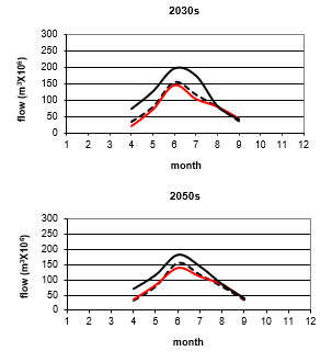
Figure 6: Historical and projected streamflow of the Arkansas River

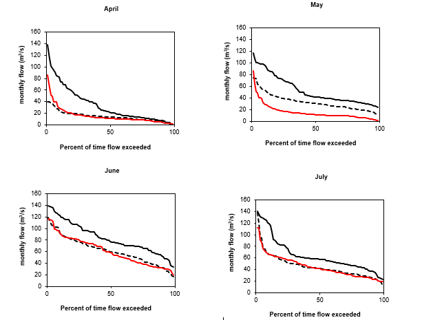
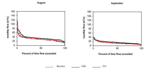Figure 7: Flow duration curves for monthly flow

6. Summary and Conclusions

This study investigated the influence of different climate phenomenon, caused by climate change, on the flow levels of the Arkansas River in USA. In order to carry out the study, time series of climate data in the future (scenarios) were extracted from two GCMs (CCC and HAD), and then plugged in a hydrologic model (ANN) to generate time series of flow. While the scenarios, produced by both models, agreed that the temperatures were likely to increase, they differed on the directionality of the change in terms of precipitation levels.

However, under the HAD-generated scenario, there is expected to be a relative increase in precipitation, resulting in increased wetness, while the CCC-generated scenario is comparatively dry and demonstrates higher variability. This variability can be attributed to annual, as well as decadal, shifts in expected climatic changes.

The results of this investigation suggest that, under the range of climate conditions studied, river flow processes are strong indicators of how climate change is impacting temperature and precipitation levels in the region. The HAD scenario in particular suggests that present flow levels are likely to be regularly exceeded in the future, especially during the peak April-July period. It further suggests that any increase in springtime flow is likely to be sizeable enough to compensate for attendant decreases in summertime flow and they further demonstrate that the historical peak flow, which used to begin in June has shifted to begin in April, extending the period of high flow levels. These results also align well with the results of other studies that explore the expected environmental effects of rising temperatures on local ecosystems in the western parts of the US [12]-[15].

The Arkansas River Basin can be considered one of the most vulnerable regions in the country when it comes to climate change. If, moving forward, precipitation levels match the projections, in terms of both magnitude and timing, they can be expected to have a significant impact that pose challenge to the water planners and managers in the region.

Conflict of Interest

No conflict of interest in publishing this paper.

Acknowledgment

The authors would like to thank VEMAP for providing the climate data.

1. E. Elgaali, Z. Tarawneh, “Effects of climate change on river flow stochastic approach,” Advances in Science and Engineering Technology International Conferences (ASET), Dubai, United Arab Emirates, 1-5, 2019, doi: 10.1109/ICASET.2019.8714549.
2. P. Mote, S. Li, Sihan, D. Lettenmaier, M. Xiao, R. Engel, “Dramatic declines in snowpack in the western US, ” Climate and Atmospheric Science, 1(2), 1-6, 2018, doi:10.1038/s41612-018-0012-1.
3. L. Dahlman, R. Lindsey, ” Climate Change: Spring Snow Cover,” Bulletin of the National Oceanic and Atmospheric Administration, 2018, Climate.gov.
4. K. E. McCluney, N. L. Poff, J. H. Thorp, G.C. Poole, M. A. Palmer, M.Williams, B.S. Williams, J.S. Baron, “Riverine macroecology: a framework for understanding the sensitivity, resistance, and resilience of whole river basins and responses to multiple human alterations,” Frontiers in Ecology and Environment, 12, 48-48, 2014, DOI: 10.1890/120367.
5. J. S. Baron, M. D. Hartman, L. E. Band, and R. B. Lammers, “Sensitivity of a high elevation Rocky Mountain watershed to altered climate and CO2,” Water Resources Research, 36(1), 89-99, 2000, 0043-1397/00/1999 WR900263.
6. D. R. Gergel, B. Nijssen, J. T. Abatzoglou, D. P. Lettenmaier, M. R. Stumbaugh, “Effects of climate change on snowpack and fire potential in the western USA,” Climatic Change, 1–13, 2017, doi:10.1007/s10584-017-1899.
7. R.W. Dudley, G.A. Hodgkins, M.R. McHale, M.J. Kolian, B. Renard, “Trends in snowmelt-related streamflow timing in the conterminous United States,” Journal of Hydrology, 547, 208-221, 2017, https://doi.org/10.1016/j.jhydrol.2017.01.051
8. T. B. Barnhart, N. P. Molotch, B. Livneh, A. A. Harpold, J. F. Knowles, D. Schneider, “Snowmelt rate dictates streamflow,” Geophys. Res 43(15), 8006-8016, 2016, DOI: 10.1002/2016GL069690.
9. G. J. McCabe, and M. P. Clark, “Trends and variability in snowmelt runoff in the western United States,” Journal of Hydrology-American Meteorology Society, 6, 467-481, 2005, https://doi.org/10.1175/JHM428.1
10. S. K. Regonda, B. Rajagopalan, M. Clark, and J. Pitlick, “Seasonal cycle shifts in hydroclimatology over the western United States,” J. Climate, 18, 372-384, 2005, https://doi.org/10.1175/JCLI-3272.1
11. I. R. Stewart, J. D. R. Cayan, and M. D. Dettinger, “Changes in snowmelt runoff timing in western North America under a ‘business as usual’ climate scenario,” J. of Climatic Changes, 62, 217-232, 2004, https://doi.org/10.1023/B:CLIM. 0000013702.22656.e8
12. C. F. Clifton, K. T. Day, C. H. Luce, G. E. Grant, S. Mohammad, J. E. Halofsky, B. P. Staab, “Effects of climate change on hydrology and water resources in the Blue Mountains, Oregon, USA,” Climate Services, 10, 9-19, 2018, DOI: 10.1016/j.cliser.2018.03.001.
13. D. Li, M. L. Wrzesien, M. Durand, J. Adam, D. P. Lettenmaier, “How much runoff originates as snow in the western United States, and how will that change in the future?,” Geophysical Research Letter, 44(12), 6163-6172, 2017, https://doi.org/10.1002/2017GL073551
14. S. Kurt, B. Katrina, M. Richard, “Shifts in historical streamflow extremes in the Colorado River Basin,” Journal of Hydrology: Regional Studies, 12, 363-377, 2017, DOI:10.1016/j.ejrh.2017.05.004.
15. D. L. Ficklin, I. T. Stewart, and E. P. Maurer, “Climate change impacts on streamflow and subbasin-scale hydrology in the upper Colorado River Basin,” PLoS One, 8(8), e71297(2013), https://doi.org/10.1371/ journal.pone.0071297
16. B. L. Harding, A. W. Wood, J. R. Prairie, “The implications of climate change scenario selection for future streamflow projection in the Upper Colorado River Basin,” Hydrol Earth Syst Sci Discuss, 9(1), 847-894, 2012, DOI: 10.5194/hessd-9-847-2012
17. D. W. Clow, “Changes in the timing of snowmelt and streamflow in Colorado:a response to recent warming,” Journal of Climate, 23, 2293–2306, 2010, https://doi.org/10.1175/2009JCLI2951.1
18. N. S. Christensen, A. W. Wood, N. Voisin, D. P. Lettenmaier, R. N. Palmer, “The effects of climate change on the hydrology and water resources of the Colorado River basin,” Climatic Change, 62(1), 337–363, 2004, DOI: 10.1023/B:CLIM.0000013684.13621.1f
19. P. Y. Groisman, R. W. Knight, and T. R. Karl, ” Heavy precipitation and high streamflow in the contiguous United States: trends in the twentieth century,” Bull. Amer. Meteor. Soc., 82(2), 219-246, 2001, DOI: 10.1175/1520-0477(2001)082<0219:HPAHSI>2.3.CO;2.
20. N. Chokkavarapu, V. R. Mandla, “Comparative study of GCMs, RCMs, downscaling and hydrological models: a review toward future climate change impact estimation,” SN Appl. Sci. 1, 1698, 2019, DOI: 10.1007/s42452-019-1764-x.
21. J. Gautam, G. Mascaro, “Evaluation of CMIP5 historical simulations in the Colorado River Basin,” International Journal of Climatology, 38(10), 3861-3877, 2018, DOI: 10.1002/joc.5540
22. M. Girotto, K. N. Musselman, R. L. H. Essery, “Data assimilation improves estimates of climate-sensitive seasonal snow,” Curr Clim Change Rep, 6, 81–94, 2020, DOI: 10.1007/s40641-020-00159-7.
23. B. S. Naz, S. C. Kao, A. Moetasim, R. Deekshai, R. Mei, L. C. Bowling, “Regional hydrologic response to climate change in the conterminous United States using high-resolution hydroclimate simulations,” Global and Planetary Change, 143, 100-117, 2016, doi: 10.1016/ j.gloplacha. 2016.06. 003
24. S. Chang, W. Graham, J. Geurink, N. Wanakule, T. Asefa, “Evaluation of impacts of future climate change and water use scenarios on regional hydrology,” Hydrol. Earth Syst. Sci., 22, 4793–4813, 2018, https://doi.org/10.5194/ hess-22-4793-2018
25. G. G. Persad, D. L Swain, C. Kouba, “Inter-model agreement on projected shifts in California hydroclimate characteristics critical to water managemen,” Climatic Change, 162, 1493–1513, 2020, https://doi.org/10.1007/s10584-020-02882-4
26. M. Haasnoot, J. Schellekens, J. J. Beersma, H. Middelkoop, J. C. J. Kwadijk1, “Transient scenarios for robust climate change adaptation illustrated for water management in The Netherlands,” Environmental Research Letters, 10 (10), 2016, DOI:10.1088/1748-9326/10/10/105008.
27. National water and climate center, Department of Agriculture. NWCC -USDA. https://www.wcc.nrcs.usda.gov/snow/snotel-wereports.html
28. T. G. F. Kittel, J.A. Royle, C. Daly, N. A. Rosenbloom, W.P. Gibson, H. H. Fisher, D. S. Schimel, L. M. Berliner, and VEMAP2 Participants, “A gridded historical (1895-1993) bioclimate dataset for the conterminous United States,” Proceedings of the 10th Conference on Applied Climatology, Reno, NV. American Meteorological Society, Boston, 219-222, 1997.
29. U.S. Geological Survey (USGS) (http://waterdata.usgs.gov/nwis/sw).
30. J. S. Patricia, S. A. Javier, P. S. Julio, P. V. David, “A Comparison of SWAT and ANN models for daily runoff simulation in different climatic zones of peninsular Spain,” Journal of water, 10(2), 192, 2018, DOI: 10.3390/ w1002 0192
31. O. I. Abiodun, A. Jantan, A. E. Omolara, K. V. Dada, N. A. Mohamed, H. Arshad, “State-of-the-art in artificial neural network applications: a survey,” Heliyon, 4(11), 2018, https://doi.org/10.1016/j.heliyon.2018.e00938.
32. I. Aichouri, A. Hani, N. Bougherira, L. Djabri, H. Chaffai, S. Lallahem, “River flow model using artificial neural networks,” Energy Procedia, 74, 1007-1014, 2015, doi.org/10.1016/j.egypro.2015.07.832.

(Click Here)