1.Introduction

In the modern manufacturing industry, technology is applied, whether it is software or hardware or a combination of the both. The 6 degrees of freedom (DOF) robotic arm is one of the most sought-after combination machinery, as is designed to be flexible for mimicking human arm functions. This is consisting of arm parts and automation control parts that are accurate and precise. However, it is like a common machine. When used for a long time or used in improper conditions, it will result in deterioration. As a result, lower accuracy does not meet the specified features, and also result in a loss of reliability. From such problems, the researchers created the idea of estimating random errors and standard uncertainty of the 6 DOF robot, which researchers have determined that the joints are the most moving parts. As a result, this is the source of the most common errors. This research develops the principles of calculating random error and uncertainty that occurs with every joint and robot.

In this research, there are two objectives: 1) Estimate the random error of each joint and estimate the robotic error. and 2) Estimate the uncertainty of each joint and estimate the robotic uncertainty. When the experiment was set up, the laser tracker was applied to measure the position of the reflector installed at the end-effector. This paper is an extension of work originally presented in 2020 IEEE 7th International Conference on Industrial Engineering and Applications (ICIEA) [1].

Over the years, many researches has been conducted in analyzing the kinematic and kinematic errors of robotic arms and other machines, such as: a study of kinematics model of Staubli RX 90 robot 6 DOF robotic arm and position of robot control was calculated and tested by writing the English Alphabet [2]. Focus on machine tool random errors in a 3D workspace and offered new models that help predict product tolerances caused by uncertainties of a machine tool [3]. The new approach with a 2D manifold that reduces the dimensionality of the workspace to improve the efficiency of error compensation for robotic machining [4]. The photogrammetry-based measurement to compensate the machining errors from parts and validated results [5]. A proposal for a guideline for a 3D-Piezo compensation mechanism unit that could quickly and accurately adjusted the spindle position to optimize robotic machining [6]. The evaluate the deviations for calculating the efficient robotic trajectory from aligned optically scanned point clouds [7] and the analysis of positioning accuracy and the kinematic parameters of robotic end-effector influenced by both internal and external temperature factors [8]. In addition, a study was proposed on improving the performance of the SEIKO D-TRAN RT3200 robot by studying the repeat control [9]. Improvement in the performance of robotic arms to have higher accuracy. Analyzed the positioning error value and then compensate for it [10]. Mathematical modeling to analyze the geometric errors of joint assembly affecting the end-effector of the 6 DOF robot was the one importance factor for robot accuracy [11]. Calibration and determination of the measurement uncertainty of robotic arms is an important issue in the confidence of the robot. There have been several research essays that discuss the principle of the measurement uncertainty such as: The kinematic error model presented by classifying the source of the error value by designing calibration methods compared to conventional calibration [12]. Applied laser interferometer to measure roundness [13]. Proposed the application of laser interferometer for calibration grade 2 gauge blocks and applied it for warhead roundness measurement [14-15]. Calibrated 6 DOF robotic arm using the Circle point analysis (CPA) method to configure a circle to measure and use the Monte Carlo method to find out the measurement uncertainty [16] and used a new method to calibrate the end-effector of 6 DOF robotic arm [17]. As mentioned above, in this research, there are the action plan is as follows: 1) Preparation of equipment and tools, 2) Learnt the involved methods and theories such as principle of the measurement method, kinematics model and the measurement uncertainties 3) experimental design and testing 4) result and conclusion.

2. Materials and Methods

2.1. Robotic arm

  Robotic arms are machines that are developed for many characteristics, but at the same time are precise and accurate. This research presents an estimate of the standard uncertainty of 6 DOF robotic arm, focusing on welding robotic arms. The robotic arm used in this research is the KUKA KR5 ARC as shown in Figure 1 and D-H parameters and joints limit as shown in Table 1.

Table 1: KUKA KR5 ARC D-H parameters

Link (n)	Link twist (αn-1)	Link length (an-1)	Link offsets (dn)	Joint angles (θn)
1	180˚	0	-400	θ1
2	90˚	180	0	θ2
3	0˚	600	0	θ3-90º
4	90˚	120	-620	θ4
5	-90˚	0	0	θ5
6	90˚	0	-115	θ6
7	180˚	0	0	180º

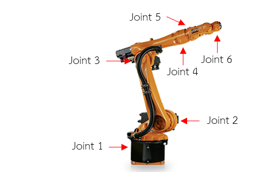Figure 1: KUKA KR5 ARC robot

2.2. Laser Tracker

Laser tracker is a 3D measurement device, which is a standard metrology in precision, accuracy and reliability. This research uses the FARO laser tracker ION model as shown in Figure 2 to measure the position of the laser reflector installed at the end-effector.

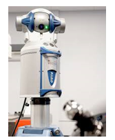Figure 2: FARO laser tracker ION model

2.3. Kinematic model

Kinematics describes the movement of object points and systems of bodies (groups of objects), regardless of the force that causes movement. Kinematics is a major part of mechanics which is often referred to as the “geometry of movement”. The kinetic problem begins by explaining the system’s geometry and declaring the initial conditions of the value, position, speed and/or acceleration within the known system. From a geometric point of view, it can locate the speed and acceleration of any unknown part of a system [18].

Robotic kinetics relies on differentials to describe the relationship between joints and links from the base to the end-effectors. The frame attached to the robotic joints is serialized like a chain. The relationship of one frame versus another frame from the bottom up will result in a conversion equation. This is the relationship of the base frame against the tool frame [19].

2.3.1. Forward kinematic

Forward kinematics are the mathematical model to compute the coordinates and directions (homogeneous conversion form) of robot end-effector positions relative to the function of the robot angles of each joints. This paper followed Denavit and Hartenberg (D-H) by choosing the reference frames in a robotic application that Jacques Denavit and Richard S. Hartenberg proposed. In this convention, the coordinate frame is attached to the joints between the two links so that one conversion involves joint [Z] and the second frame is linked to the link [X], converting coordinates with serial robots that contain n links to the robot’s equation format. D-H convention determines each conversion A_n with a multiple of fundamental conversions, respectively. The transformation matrix can be written as follows:

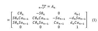where, A_n is the homogeneous matrix that describes the movement of the frame of each contiguous joint (n-1 and n). θ_n is the joint angle of the ith joint, d_n is the link offset of the ith joint, a_n is the link length of the ith joint, and α_n is link twist of the ith joint. Sθ_n = S_n = sin(θ_n), Sα_n = sin(α_n), Cθ_n = C_n = cos(θ_n) and Cα_n = cos(α_n).

The parameters were replaced in Table 1 in (1), and multiplied all the matrixes in order. It is the last matrix that shows the position and direction of the end-effector compared to the base can be displayed as follows:

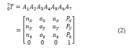In this research, the linear position of end-effector is determined, which shows the position in the coordinates x, y, and z, as shown in (3).

P_x = C₁[a₁ + a₂C₂ + S₂₃(a₃ + d₆C₄S₅) – C₂₃(d₄ + d₆C₅)]

                + d₆S₁S₄S₅

   P_y = –S₁[a₁ + a₂C₂ + S₂₃(a₃  + d₆C₄S₅) – C₂₃(d₄ + d₆C₅)]

                + d₆C₁S₄S₅

P_z = –d₁ – a₂S₂ + C₂₃(a₃ + d₆C₄S₅) + S₂₃(d₄ + d₆C₅)       (3)

2.3.2. Inverse kinematic

In the previous section, the robot forward kinematics are the mathematical equations, used to calculate the position and direction of the end-effector frame compared with base frame when the variables joints (q₀, q₁, q₂,…, q_n) are known. On the other hand, to know the variable joints (q₀, q₁, q₂,…, q_n), when determining the homogeneous matrix at the end-effector frame compared to the base frame (), the resulting relationship is called inverse kinematics.

For general cases in robotics, the inverse kinematics calculation of the robot is more complex than the forward kinematics problems because the results can occur in 3 different ways consisting of no solution, unique solution, and many solutions.

2.3.3. Jacobian matrix

The Jacobian matrix is a matrix that shows the relationship between the error of the end-effector and the 6 joints error of the robot. The Jacobian matrix can be found in the analysis of the forward kinematic, as shown in (4).

  dX = Jdθ_i                                            (4)

where,    dθ_i are the angle errors of 6 axis (i=1, 2, 3,…,6).

                J is Jacobian matrix.

Jacobian’s pattern is in the form of a 6×6 matrix, which is based on (5):

J_6×6  = [J₁ J₂ J₃ J₄ J₅ J₆]         (5)

The six joints of the robot are all revolute (R). Therefore, the Jacobian matrix can be calculated as follows:

where,  z_i-1 is the value of the top 3 elements in column 3 of the matrix

o_i is the value of the top 3 elements in column 4 of the matrix

When a robot moves, the linear position error for x, y and z direction of the end-effector, can be written in a partial derivative of equation 3 relative to the angle in each of the changing joints. The Jacobian components that are affected by the x, y and z linear position of end-effector in Jacobian matrix as follows:

J₁₁ = – S₁ [a₁ + a₂C₂ + S₂₃(a₃ + d₆C₄S₅) – C₂₃(d₄ + d₆C₅)]   

         +d₆C₁S₄S₅

J₁₂ = C₁[C₂₃(a₃ + d₆C₄S₅) + S₂(d₄ + d₆C₅) – a₂S₂]

J₁₃ = C₁[C₂₃(a₃ + d₆C₄S₅) + S₂₃(d₄ +d₆C₅)]

J₁₄ = d₆S₅(C₁S₂₃S₄ + S₁C₄)

J₁₅ = d₆(C₁S₂₃C₄C₅ + C₁C₂₃S₅ + S₁S₄C₅)

J₁₆ = 0

J₂₁ = –C₁[a₁ + a₂C₂ + S₂₃(a₃ + d₆C₄S₅) – C₂₃(d₄ + d₆C₅)] 

         – d₆S₁S₄S₅

J₂₂ = S₁[a₂S₂ – C₂₃(a₃ + d₆C₄S₅) – S₂₃(d₄ + d₆C₅)]

J₂₃ = S₁[–C₂₃(a₃ + d₆C₄S₅) – S₂₃(d₄ + d₆C₅)]

J₂₄ = d₆S₅(S₁S₂₃S₄ + C₁C₄)

J₂₅ = –d₆(S₁S₂₃C₄C₅ + S₁C₂₃S₅ – C₁S₄C₅)

J₂₆ = 0

J₃₁ = 0

J₃₂ = – [S₂₃(a₃ + d₆C₄S₅) – C₂₃(d₄ + d₆C₅) + a₂S₂]

J₃₃ = –S₂₃(a₃ + d₆C₄S₅) + C₂₃(d₄ + d₆C₅)

J₃₄ = –d₆C₂₃S₄S₅

J₃₅ = –d₆(S₂₃S₅ – C₂₃C₄C₅)

J₃₆ = 0

2.4. Principle of measurement the random error of individual robotic joints method

In this research, the principle of the proposed measurement method measures the positions the end-effector in 3 dimensions system (x, y, z) that is affected from the rotation of a joint when the others are locked. Figure 3 shows an example of the measurement principle of joint 2. After the measurement system setup, the program instructs the end-effector to move to the specified position (P₁, P₂, P₃,…, P_n). The laser tracker measures the position according to the specified cycle, the identification of rotation plane and rotation center are shown in section 2.4.1 and 2.4.2.

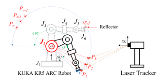Figure 3: Basic principle of the measurement method for J₂                                 random joint error setting

2.4.1. Identification of rotation plane

Identifying a rotating plane of the robotic arm joints aims to create a circular arc from the rotation of the joints measured in the Cartesian area. This arc has a measurement points m. The rotation plane in the Cartesian space can be calculated as follows:

z = Ex + Fy + G                               (7)

The previous equation is where x, y and z are coordinates points in the rotation plane.  E, F and G are the rotation plane coefficients.

In the rotation plane, the adjustment of the measurement point (x_i, y_i, z_i) when k=1, …, m is derived from the minimization problem as follows:

2.4.2. Identification of rotation center

In theory, the trajectory of the m point in the arc of the circle of a rigid body, this circle plane is perpendicular to the fixed axis. However, in the practice, there are some factors such as vibration during rotation and the non-standard assembly etc. So, that result in the trajectory of the m points may not be completely circular and assume that the theoretical circular and circle trajectory have very few deviations, thereby, a circle equation from the equation (9) is used to fit these points. So, the rotation plane of robotic arm joints can be calculated. Using the least square method was done in order to identify the circle on the circle plane. A standard form of a circle equation is as follows:

(x – x_c)² + (y – y_c)² = r²                               (9)

The previous equation is where (x_c, y_c) is the rotation center. r is the radius of the circle. From (3) can be rewritten as follow:

w = x² + y² = Ax + By + C                        (10)

The previous equation is where A, B and C are the coefficients of the circle center in 3D system. Then, there are the sets of measured (x_i, y_i, z_i) when i=1, 2, 3, …, m is derived from the minimization problem as follows:

2.4.3. Experiment setup

This system consists of 3 important parts: 1) robotic arm. 2) laser tracker. and 3) installation of the reflector at the end effector as shown in Figure 4.

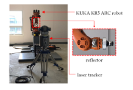Figure 4: The 6 DOF KUKA KR5 ARC robot experimental setup

The installation was used to measure a KUKA KR5 ARC robot with a FARO laser tracker ION model. Positional measurement was performed with a reflector installed at the end effector of the robot by measuring any joint i, other joints are locked to stay with that. All measurements were measured at the temperatures between 30 to 34 °C. The position of the robotic base frame and the coordinate measurement frame of the laser tracker was set in alignment. The measurement processes are as follows:

• Assign the end-effector move to the first position P1.
• Unmeasured joints are locked from moving. After that measured the points P₁, P₂, P₃, …, P_n are fitted with a plane in the Cartesian space.
• On the determined plane, specifies the points on the arc of the circle P₁, P₂, P₃, …, P_n and determines the center of the circle O.
• Measured 30 times repeat for every points m.

2.5. Evaluation for Measurement Accuracy

 In a high-accuracy and high-precision measurement system to increase measurement and reliable confidence levels, measurement accuracy is required to increase the confidence and reliability of the measurement. Therefore, measurement accuracy assessment is required. This evaluation compares the deviation (errors) between frame {E_i} and frame {E_i‘} where, frame {E_i} is calculated by the proposed method and frame {E_i‘} is calculated by forward kinematic of robotic arm.

2.5.1. Joint errors

Joints errors are due to repeatability of measurement and can be calculated as the difference between actual (measurement) and nominal angle. The position of end-effector is converted to the angle of each joint with inverse kinematics. The actual angle as shown in (12-17):

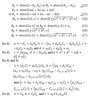
Therefore, the joint errors can be calculated as follow:

where,    θ_in are the nominal angle.

                θ_ia are the actual (measurement) angle.

                g is number of measurement points.

                i are the robotic joints (i=1, 2, 3, …, 6).

2.5.2. Position errors

In this research, the linear position error for x, y and z direction of the end-effector (dx, dy, dz) are determined. Therefore, the position errors in the x, y and z axes at the end-effector as shown in (19-21) respectively.

dx = J₁₁d?₁ + J₁₂dθ₂ + J₁₃d?₃ + J₁₄d?₄ + J₁₅d?₅ + J₁₆d?₆  (19)

dy = J₂₁d?₁ + J₂₂dθ₂ + J₂₃d?₃ + J₂₄d?₄ + J₂₅d?₅ + J₂₆d?₆  (20)

dz = J₃₁d?₁ + J₃₂dθ₂ + J₃₃d?₃ + J₃₄d?₄ + J₃₅d?₅ + J₃₆d?₆  (21)

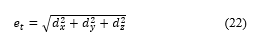
From that (19-21) can calculate the total error at the end-effector as follows:

2.6. Measurement uncertainty

In metrology, measurement uncertainty is an expression of statistical distribution of values caused by measured quantities. Therefore, measurement uncertainty is used in combination with the measurement results to reflect the actual value of the measurement quantity. Especially, when the measurement results are applied to various quality criteria, the results must be applied to the quality criteria. According to international agreements, this uncertainty is based on probability and shows the incomplete of the quantity and it is a non-negative parameter.

Multiple repetitive measurements and calculating standard deviations from re-measuring are among the most common practices in estimating measurement uncertainty. Whether it is a full or partial measurement, it can be repeated. The estimation of the uncertainty received is a standard deviation of the repetitive measurement results, which is a statistical process. It is called type A uncertainty. The type B uncertainty is estimated from other deviation source such as material certificates, specifications, and long-term experience-based assessments [20].

The Expression of Uncertainty and Confidence in Measurement, M3003 [21] and Fundamental Parameter and Application describes how to calculate standard uncertainty.

2.6.1. Type A uncertainty

Type A uncertainty is estimated using statistical principles. By performing measurements, conditions are subject to repeated measurement conditions to see the original iteration or view the distribution of the measured average. The arithmetic mean, or average, of the results should be calculated. If there are n independent repeated values for a quantity Q then the mean value  is given by:

Then the estimated fragmentation of data is calculated from the standard deviation of the n values can compute as follows:

Equation (24) gives the standard deviation for sampling from all populations. However, based on the results of a single measurement sample, approximate, s(qj), can be made from the standard deviation σ of the entire population of possible values from the relation:

The average q will be derived from the exact sample number of n and, therefore, its value will not be the exact average if the infinite sample number is taken. This uncertainty is called the standard deviation of the mean that can compute as follow:

2.6.2. Type B uncertainty

Estimating type B uncertainty is the other way around. In other words, it uses information from various sources that are academically reliable to consider the assessment. The error element from a source called the systematic error is valued as a type B uncertainty. Therefore, estimating the type B uncertainty requires a lot of knowledge of measurement techniques. In order to be able to identify a source of uncertainty, much of the systematic error is complete. The estimation of uncertainty needs to consider the source of uncertainty values as follows:

• Deviation Instability compared to the reference standard stipulated in the reported calibration uncertainty.
• Calibration of measuring instruments includes accessories and any drift or instability in measuring instruments or readings.
• Resolution and uncertainty during measurement.
• The operational procedure.
• Mistakes caused by the operator.
• The effects from environment.

2.6.3. Combined uncertainty

The type A and B uncertainty values are part of the overall measurement uncertainty value, which can be calculated for the combined standard uncertainty as shown in (27):

where u_c(y) is the combined uncertainty, c_i is the sensitivity coefficient and u(x_i) is the standard uncertainty.

2.6.4. Expanded uncertainty

The combined uncertainty that is approximated is considered to have a certain level of confidence which is not suitable enough for laboratory use. Therefore, it is necessary to multiply combined uncertainty with coverage factor k. The expanded uncertainty as follows:

U = k.u_c(y)                                     (28)

2.6.5. Robot uncertainty

In this research, the uncertainties position errors for x, y and z direction of the end-effector (U_x, U_y and U_z)  are determined. Therefore, the uncertainties position errors in the x, y and z axes at the end-effector (U_x, U_y and U_z) as the function of joint uncertainty (U₁, U₂, U₃, U₄, U₅ and U₆) are shown in (29-31) respectively.

U_x = J₁₁U₁ + J₁₂U₂ + J₁₃U₃ + J₁₄U₄ + J₁₅U₅ + J₁₆U₆      (29)

U_y = J₂₁U₁ + J₂₂U₂ + J₂₃U₃ + J₂₄U₄ + J₂₅U₅ + J₂₆U₆      (30)

U_z = J₃₁U₁ + J₃₂U₂ + J₃₃U₃ + J₃₄U₄ + J₃₅U₅ + J₃₆U₆      (31)

From that (29-31), it can calculate the total uncertainty at the end-effector as follows:

3. Results

The research focuses on the study estimating the standard uncertainty of 6 DOF KUKA KR5 ARC robot, considering the 3 key parts of which parameter values used in calculations derived from the experiment as shown in section 3.1-3.2 consist of robotic errors and robotic uncertainties.

3.1. Robotic error

The errors of the robot in this research are divided into two parts: joint errors and position errors.

3.1.1. Average Joint errors

Based on the experiments measuring data from section 2.4, the average joint errors are calculated according to (18).

      Joint 1 average error (d?₁) equals 0.101º.

      Joint 2 average error (d?₂) equals –0.287º.

      Joint 3 average error (d?₃) equals 0.070º.

      Joint 4 average error (d?₄) equals –0.097º.

      Joint 5 average error (d?₅) equals 0.026º.

      Joint 6 average error (d?₆) equals 0.140º.

3.1.2. Average Position errors

When average joint errors are known, the average position errors at the end-effector in x, y and z axis can be calculated according to (19-21).

Average Position error in x axis (d_x) equals –0.357 mm.

Average Position error in y axis (d_y) equals –0.303 mm.

Average Position error in z axis (d_z) equals 0.383 mm.

So, instead of position errors at the end-effector in x, y and z axis in (21), the average robot error (e_t) is equal to 0.605 mm.

3.2. Robotic uncertainty

The uncertainties of the robot in this research are divided into two parts: joint uncertainties and position uncertainties.

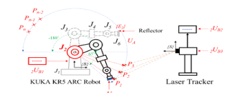Figure 5: Basic principle of the measurement method and sources of uncertainty

3.2.1. Joint uncertainties

The research is based on the principle of the measurement method and then calculates the average position errors and the standard deviations of position errors of the robotic joints. These errors show the accuracy, and the standard deviations show the precision of the joints. After that, these values are used to determine the type A standard of joints 1 to 6 of the robot.

Figure 5 shows the basic principle of the measurement method and the sources of uncertainty. In this research, the sources of uncertainty consist of five sources, that uncertainties are type A uncertainty (_iU_A) and four sources of type B uncertainty (_iU_Bj):

where,    _iU_A are the uncertainty from repeatability.

_iU_B1 are the uncertainty from resolution of the robot.

                _iU_B2 are the uncertainty from resolution of laser tracker.

_iU_B3 are the uncertainty from accuracy of laser tracker.

_iU_B4 are the uncertainty from thermal effect at the reflector fixture.

i are the robotic arm joints.

j are the number of the sources of uncertainty.

Table 2 provides a preview of the sources of the uncertainty and the calculation of the total uncertainty of the 1st joint. The uncertainty of each joint are as follows:

The uncertainty of joint 1 (U₁) equal ±0.204º.

The uncertainty of joint 2 (U₂) equal ±0.149º.

The uncertainty of joint 3 (U₃) equal ±0.076º.

The uncertainty of joint 4 (U₄) equal ±0.126º.

The uncertainty of joint 5 (U₅) equal ±0.140º.

The uncertainty of joint 6 (U₆) equal ±0.115º.

3.2.2. Position uncertainties (Robot uncertainty)

When the uncertainties of each joint are known. The uncertainties in x, y and z axis at the end-effector can be calculated according to (29-31), the results as the follow:

The uncertainty in x axis (U_x) equal ±0.225 mm.

The uncertainty in y axis (U_y) equal ±0.613 mm.

The uncertainty in z axis (U_z) equal ±0.366 mm.

So, instead of position uncertainties at the end-effector in x, y and z axis in (32), the average robot uncertainty (U_t) is equal to ±0.748 mm.

The research results showed that the KUKA KR5 ARC robot used in the experiment had the average robot error which (e_t) is equal to 0.605 mm. and with the average robot uncertainty (U_t) is equal to ±0.748 mm. Then, examples of four test points (P₁, P₂, P₃ and P₄) are used to determine the estimated error and uncertainty in each joint from propose model. The position errors and position uncertainties at the end-effector in x, y and z axis can be calculated according to (19–21) and (29–31). The results of the estimated robot position errors and the position uncertainty are shown in the Table 3.

4. Discussion

Objective 1: Measure random errors of each joint and the robot end-effector linear random error in x, y and z direction and average error can be calculated. When comparing the robot error with the specified accuracy, the robot error was found to be slightly higher than the accuracy value. The results of the research process can be compensated in the control system, as it can reduce the error value.

Objective 2: Estimate the uncertainty of each joint and estimate the robot uncertainty. The results show that the uncertainty of each joint at 95% confidence level was quite high and when calculating the average uncertainty of the robot it was quite high too. The high average uncertainty will result in a difference of the robotic error. The biggest uncertainty is the uncertainty from repeatability. It was between 86.21% and 94.48%. This suggests that the uncertainty from repeatability has a significant effect on the total uncertainty, so it is appropriate to consider this factor.

Table 2: The standard uncertainty of joint 1

Type	Value (degree)	Distribution	Divisor	Uncertainty contribution ui (degree)	Sensitivity coefficient ci	Effective DOF Veff
1UA	0.1019	Normal	1	0.1019	1	20
1UB1	0.0019	Rectangular		0.0011	1	∞
1UB2	0.0095	Rectangular		0.0055	1	∞
1UB3	0.0035	Rectangular		0.0020	1	∞
1UB4	0.0002	Rectangular		0.0001	1	∞
1UC		–		0.0083		∞
1Ur		Normal k=2		0.2042		∞

Table 3: The estimated position errors and uncertainties for the example of four test points

Points	Target position (mm)			Position errors (mm)				Position Uncertainties (mm)
	x	y	z	dx	dy	dz	et	Ux	Uy	Uz	Ut
P1	125	125	125	– 0.033	– 0.012	0.445	0.447	±0.164	±0.163	±0.177	±0.291
P2	225	225	225	– 0.118	0.182	0.414	0.467	±0.164	±0.163	±0.177	±0.291
P3	225	25	225	– 0.125	– 0.077	0.465	0.488	±0.159	±0.161	±0.185	±0.292
P4	25	25	25	– 0.050	– 0.093	0.199	0.225	±0.168	±0.159	±0.178	±0.292

Therefore, the results from Table 3, the position errors and the uncertainties of all test points within the robot moving space are calculated and estimated by the proposed method and model. Therefore, the position error tolerance of each required moving target point must be smaller than the position errors and the uncertainties that are estimated from this proposed model.

5. Conclusions

In this research, it describes the method of testing and experimenting to calculate the errors of each joint, and calculating the actual angle of their joint to compare with a nominal joint angle. The Jacobian matrix was applied to estimate the robot position error. The estimation of the uncertainties of each joint by using Jacobian matrix was done to estimate the robot position uncertainty. The research results showed that the KUKA KR5 ARC robot used in the experiment average robot error (e_t) was equal to 0.605 mm. and with the average robot uncertainty (U_t) being equal to ±0.748 mm.

The example of the four test points (P₁, P₂, P₃ and P₄) determined the estimated error and uncertainty in each joint from proposed model. The position errors (e_t) was 0.447mm, 0.467 mm, 0.488 mm and 0.225 mm respectively. The position uncertainty (U_t) was ±0.291 mm, ±0.291 mm, ±0.292 and ±0.292 mm. The position errors and the uncertainties of all test points within robot space moving were calculated and estimated by the proposed method and model. Therefore, the position error tolerance of each required test point must be smaller than the position errors and the uncertainties that are estimated from this proposed model.

Acknowledgement

This research was supported by the National Science and Technology Development Agency, Thailand, Project no. FDA-CO-2560-4832-TH.

1. A. Loungthongkam, C. Raksiri “A Development of Mathematical Model for Predictive of The Standard Uncertainty of Robot Arm” International Conference on Industrial Engineering and Applications (ICIEA)., 2020. https://doi.org/10.1109/ICIEA49774.2020.9101979
2. B. Panomruttanarung, W. Pornsukvitoon, J. Pakkawanit “A Study of Forward and Inverse Kinematics for 6-Link Robot Arm (Staubli RX90)” The Journal of KMUTNB., 27(2), 241-252, 2017. DOI: 10.14416/j.kmutnb.2017.03.013
3. K. G. Ahn, D. W. Cho “An analysis of the volumetric error uncertainty of a three-axis machine tool by beta distribution” International Journal of Machine Tools and Manufacture., 40(15), 2235-2248, 2000. https://doi.org/10.1016/S0890-6955(00)00048-1ff
4. Z. Weidong, L. Guanhua, D. Huiyue, K. Yinglin “Positioning error compensation on two-dimensional manifold for robotic machining” Robotics and Computer Integrated Manufacturing., 59, 394-405, 2019. https://doi.org/10.1016/j.rcim.2019.05.013
5. J.D. Barnfather, M.J. Goodfellow, T. Abram “Development and testing of an error compensation algorithm for photogrammetry assisted robotic machining” Measurement., 94, 561-577, 2016. https://doi.org/10.1016/ j.measurement.2016.08.032
6. U. Schneider, M. Drust, A. Puzik, A. Verl “Compensation of Errors in Robot Machining with a Parallel 3D-Piezo Compensation Mechanis” Procedia CIRP., 7, 305-310, 2013. https://doi.org/10.1016/j.procir.2013 .05.052
7. J.D. Barnfather, T. Abram “Efficient compensation of dimensional errors in robotic machining using imperfect point cloud part inspection data” Measurement., 117, 176-185, 2018. https://doi.org/10.1016/j.measurement. 2017 .12.021
8. R. Li, Y. Zhao “Dynamic error compensation for industrial robot based on thermal effect model” Measurement., 88, 113-120, 2016. https://doi.org/10.1016/j.measurement.2016.02.038
9. P. Roopyai, B. Panomruttanarung, “Positioning Error Reduction in Robotic Manipulator SEIKO D-TRAN RT3200 Using Repetitive Control” The Journal of KMUTNB., 28(2), 299-312, 2018. DOI: 10.14416/j.kmutnb.2018.03.006
10. Y. Zeng, W. Tian, W. Liao, “Positional error similarity analysis for error compensation of industrial robots” Robotics and Computer-Integrated Manufacturing., 42, 113-120, 2016. https://doi.org/10.1016/j.rcim.2016.05.011
11. C. Raksiri, K. Pa-im, S. Rodkwan, “An Analysis of Joint Assembly Geometric Errors Affecting End-Effector for Six-Axis Robots” Robotics., 9(2), 1-13, 2020. https://doi.org/10.3390/robotics9020027
12. L. Ma, P. Bazzoli, P. Sammons, R.G. Landers, “Modeling and calibration of high-order joint-dependent kinematic errors for industrial robots” Robotics and Computer-Integrated Manufacturing., 50, 153-167, 2018. https://doi.org/10.1016 /j.rcim.2017.09.006
13. T. Dokyor, “An application of Michelson laser interferometer for roundness measurement” M.S. Thesis, Kasetsart University, 2008.
14. A. Loungthongkam, “A study an application of Michelson laser interferometer for calibration block gauges” M.S. Thesis, Kasetsart University, 2011.
15. A. Loungthongkam, “High precision technique of laser interferometer for warhead roundness measurement” Journal of Industrial and Intelligent Information., 3(2), 158-162, 2015. doi: 10.12720/jiii.3.2.158-162
16. J. Santolaria, “Uncertainty estimation in robot kinematic calibration” Robotics and Computer-Integrated Manufacturing., 29(2), 370-384, 2013. https://doi.org/10.1016/j.rcim.2012.09.007
17. H.-N. Nguyen, J. Zhou, H.-J. Kang, “A New Full Pose Measurement Method for Robot Calibration” Sensors., 13(7), 9132-9147, 2013. https://doi.org/10.3390/s130709132
18. A.A. Shabana, Dynamics of Multibody Systems, Cambridge University Press, 2013.
19. W. Toojinda, Industrial Robot Analysis and Control, Chula Press, 2017.
20. JCGM, Evaluation of measurement data – Guide to expression of uncertainty in measurement, Joint Committee for Guides in Metrology, 2008.
21. United Kingdom Accreditation Service, The Expression of Uncertainty and Confidence in Measurement, M3003, 2019

(Click Here)