1.Introduction

This paper is an extension of work originally presented in 2020 International SAUPEC/RobMech/PRASA Conference [1]. Haptic feedback control systems containing human- in- the- loop (HITL) is relatively a young field of research, that display the interaction between human-machine systems. A typical bilateral teleoperation system consisting of the master device (human operator), communication channel and slave teleoperator, provide human operator’s necessary interface and the experience of ‘telepresence’ [2, 3]. In simple text, the human perceives direct control and manipulation of the environment with their own hands, which is achieved by having their actions mediated physically by means of a robot, communication channel and control systems (i.e., controller), by providing the haptic sensing feedback signals (mostly interaction forces and position constraints) to the operators. Thus, the human operator can execute tasks remotely without physically being present there. Potential applications of teleoperation systems include highly specialized professions like telesurgery, mining, micro, and nanoparticles handling and artificial intelligence to name just a few [4]. These operations are performed globally, mainly to aid and assist the population with special needs.
The block diagram shown in Figure 1 gives a control system viewpoint of haptic teleoperation system. The main purpose of this system is the operator’s ability to interact with the remote environment via haptic feedback. In this haptic teleoperation system, a human operator gets the feel of telepresence in the form of force operation and vibrations (sensations) from the haptic interface system, for instance, a simlulator. Thus, the movement of the human arm is based on the haptic feedback signals received from the haptic interface device. Accordingly, the human arm will send force and position signals to the controller (highlighted in the top red circle) which will forward the modified force and position signals to the robot system. The robot will then exert the received control signal to the concerned object present in the remote environment. The measured signals (force, position, and vibration) are then fed back to the haptic interface (highlighted in the bottom red circle) resulting in haptic feedback and HITL system. Thus, the human operator feels they are directly executing control operation of the remote side themselves.

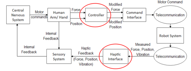Figure 1: Control system viewpoint of haptic teleoperation system

In teleoperation systems, stability and transparency are both critical properties and conflicting to each other [5]. One of the main concerns relating to control systems design, is to achieve a decent tradeoff between these two contrasting goals. Stability can be achieved using Proportional integral derivative (PID) controls [6], wave-variables based passivity control [7] and time-domain passivity approach [8]. Whereas transparency is related to the human operator’s potential to sense the slave side interaction with the environment. To enable this, force sensors are installed at the end effector providing force feedback control. Conversely, these force sensors impose measurement limitations due to their high cost, restricted area of contact and noise/ disturbances in the environment. Hence, disturbance observers were introduced [9]. On the contrary, these observers do not consider specific knowledge of the system like unmodelled dynamics and parameter uncertainties, resulting in narrowing the effectiveness of model-based controllers. Thus, these shortcomings have motivated the application of a model independent approach in the domain of bilateral teleoperation systems. Hence, an Active disturbance rejection control (ADRC) has been proven effective to tackle the limitations of both PID and model-based approaches [10,11]. ADRC’s dynamic structure components, such as, the ESO (Extended state observer) and TD (Tracking differentiator), are used to compensate for internal and external disturbance(s) respectively. Therefore, the total system from the outside looks linear. The ADRC takes into account the time-varying nature of the system, unlike the PID controller, that considers particular time instants only. References [12–14] are survey papers that review the development of ADRC from its early beginning, along with, the controller’s analysis being conducted from its methodology and theoretical perspective.
This paper aims to addresses and release the above mentioned constraints related to model- based approaches in control theory. This can be attained by introducing a model free approach (ADRC controller) for the physical interface platform (HMI) developed for this research. The objective of this paper includes the study of the disturbance rejection performances and control variable responses of the ADRC and PI controllers. The former provides a better understanding on the system response curves obtained, whereas the latter depicts more information on controller behaviour. Contributions of this paper include the algorithmic innovation of the ADRC controller and development of a controlled object that serves as a movable two- dimensional (2D) interface platform. Based on this platform, we propose an ADRC for the system shown in Figure 1. Furthermore, this paper focusses on the integration of the designed controller with the human machine interface platform, followed by their experimental analysis and comparison with the previously obtained PI controller results in [1]. This integration and analysis serves as the main focal point of the paper. Thus, by this comparison, the effectiveness of the total proposed system is measured. All the simulations will be conducted via MATLAB and Simulink in this study. Apart from MATLAB/ Simulink, experimental analysis for ADRC based applications have been conducted using other softwares, like LabView, Scilab/ Xcos and OpenPCS, to name a few.
The rest of the paper is structured in this way: Initially, the related work is briefly explained in Section 2, subsequently the proposed hardware platform is addressed in Section 3. Furthermore, Section 4 discusses the design and simulation of an ADRC controller, followed by results and discussions in Section 5. Lastly, Section 6 closes the paper.

Related Works

ADRC Controller

For almost a century, the PID controller has dominated the control technology to meet the ever-increasing demands of the automation industry. However, the PID controller design being system-dependent falls under the category of error-based empirical design paradigm (EDP) [11]. Tuning of such controllers is challenging due to model mismatch between the actual system and approximate model. Other challenges include computational error, noise deterioration caused by derivative control, performance degradation in the control law (linear weighted sum) and complications by integral control due to accumulation of errors [10]. These conditions necessitated the introduction of a special type of nonlinear controller being system model-independent, called the ADRC. This controller possesses features of strong robustness, fast response speed, high accuracy control, minimum overshoot (smooth curve) and capability to estimate and compensate the overall effects of uncertainties and is thus minimized. These uncertainties include unknown plant dynamics, external disturbances and internal disturbances, in real-time. The capability to control uncertainties in a given system is one of the principal concerns in the field of modern control theory. The ADRC design was first proposed in [15], followed in 1998 [16], for plants with a large number of uncertainties. The same was introduced in [17], followed by an extension in [11]. An adequate transient response is attained using an ADRC design, which possesses a relatively simple framework.

Disturbance Rejection Mechanism

The existing paradigms in the field of control engineering, are the Modern Control Paradigm (MCP) (model-based approach) and error-based Empirical Design Paradigm (EDP) (classical trial and error approach) [11]. But there is a significant gap between theory and practice in the field of feedback control engineering. This calls for a paradigm shift introducing a new paradigm, namely, Disturbance Rejection Paradigm (DRC) [18].
The basic idea of ADRC can be put straight in the following train of thoughts. Firstly, cascade integral design of the canonical (ideal) configuration of the plant. Secondly, portion of the plant that is distinct from the ideal form can be called the ‘total disturbance’, and is rejected. This includes internal disturbance (i.e. variations in plant dynamics) and external disturbance (i.e. arises from the environment). Lastly, estimate and compensate the total disturbance using an extended state observer (ESO), so as to reduce the nonlinear time-varying system to the canonical form. In short, two main characteristics of modern control theory on which the fundamentals of ADRC are set: Firstly, the concept of canonical form; Secondly, the objective of a state observer [12]. Thus, with such a unique design concept, ADRC provides exceptional outstanding solutions to various pressing problems in the engineering field. Thus, practical applications of ADRC include robot motion control and aerial robotic systems [19], control tool for practitioners [20], control of humanoid robot [21], quadrotor helicopter [22], in several chemical processes, MEMS systems and power converters [23,24], to name a few.
Haptic Feedback Control
Over the last four decades, several bilateral teleoperation architectures were developed serving as the key technology for human interaction with the remote environment, by supplying the operator with haptic feedback. This haptic feedback control improves the quality of human-robot interaction, on the other hand, stability and transparency parameters are greatly affected due to time delay and packet loss in the communication channel, between the master side (operator) and slave side (remote robot interaction with the environment), as shown in Figure 2.

Figure 2: A basic haptic teleoperation system

Some of the important teleoperation architectures, along with their methods, studied and analysed in the past include Wave-variable (WV) approach [25,26], Time-domain passivity approach (TDPA) [27,28], and Model- mediated teleoperation (MMT) approach [29]. A detailed survey on the bilateral teleoperation algorithms and model-based control architectures for haptic interfaces is given in [3]. Such model-based methods represent input-output relationships using mathematical expressions, like the state-space model, Lagrange model, and transfer function model. They are also represented using various control laws, for example, the proportional integral (PI), proportional derivative (PD), PID, model predictive, sliding mode, and energy-based controllers [8,30].
The haptic teleoperation system control and design experience certain shortcomings, such as, uncertainties related to the communication channel and human operational dynamics, along with unsteady human operator decisions [31]. These uncertainties are time-varying and distinctive among individuals. Such inaccuracies make the model-based controller operation challenging and stimulate the use of model-free controllers, like the ADRC for smooth operations [10]. Thus, ADRC can contribute to the development of applications in connection with feedback contro1l systems in man- machine interface systems. Recent studies on ADRC controller for teleoperation systems based on distinct parameters, and for nonlinear systems, have been explained in [32] and [33,34] respectively.
Hardware design and modelling
Proposed Hardware Platform
The basic idea behind the platform shown in Figure 3, is to manoeuvre the operating handle in a rectangular coordinate system.

Figure 3: Experimental setup of the assembled hardware platform- 2 degree of freedom (2 DOF)

Mechanical components of the HMI design

Mechanical and electrical components constitute the experimental platform. The mechanical components used are stated in this subsection. The operating handle is a three- dimensional (3D) printed object, obtained using a designing software called Onshape. Both X-axis and Y-axis have a ball screw feed drive system (SFU1605) aligned parallel to each of the axis, with the operating handle assembled over the lead screw system. The ball-lead screws and nut dimensions are 600mm (length) x 16mm (diameter) x 5mm (pitch). Ball screw nuts provide the required linkage between the lead screws and the operating handle. Hence, ball lead-screw’s rotational motion is transformed to operating handle’s linear translation motion. As seen in Figure 3, two pairs of linear guide rails of dimensions 600mm (length) x 4mm (width) hold up the handle and screws. The guide rails used are called the Igus W series (WS-10-40-600), which possess benefits like low wear and tear, low friction, low noise system, and requires no maintenance being resistant to dust and dirt. The 3D printed carriages that firmly hold both ends of the lead screws, together with the sliding rails, are all mounted on a levelled surface. The end supports used for the ball screw (SFU16XX – BK 12 + BF 10) contains two parts, one for the front and the other for the rear of the lead screw. The fixed part is 10mm in diameter, whereas the floating part is 12mm in diameter. Also includes circlips and deep groove ball bearings. A DC motor mounted on one end-support component, and the motor shaft mechanically connected to the lead screw, help to drive the lead screw system.

Electrical components of the HMI design

The electrical components used in the experimental setup are explained in this subsection. As seen in Figure 3, a DC motor shaft equipped with an encoder is incorporated at one end of both the lead screws. The motors chosen are called the Metal Gearmotor 75:1 (gear ratio), with a 48 CPR quadrature encoder integrated on each motor, which provides 3592 counts per revolution of the gearbox’s output shaft. Size of the motor is 25mm (diameter) x 66mm (length), with a shaft diameter of 4mm. These motors are intended for comfortable operation in the 3- 9V range. The encoders are connected to the Arduino MEGA 2560 board. Both motors are provided with a specific motor driver called the BTS7960 High Power H- Bridge motor driver. The motor driver has the following specifications, 43A of maximum current and input voltage range of 6V to 27V. According to the inout voltage received from the Arduino board, the motor drivers will adapt to these incoming signals, and then apply the appropriate voltage to the motor. The system contains two ACS714 current sensors, one for each motor driver, to aid in measuring the strength applied on the operating handle.
On accomplishing the hardware installation, signal transmission between MATLAB and the proposed interface system (HMI) was performed using Arduino 2560. This Arduino board was powered by an external power supply. Currently, only a single axis movement of the lead screw drive system is considered in this paper.

Mathematical Modelling of the Assembled Hardware Platform

Two of the single-axis electro-mechanical platform shown in Figure 3 are coupled together to implement the 2D movement. Torque (T_M) generated by the DC motor is transmitted to the ball screw shaft via coupling, which in turn causes the operating handle to move. Transmission ratio ‘i’ of ball screw system is defined as the distance travelled ‘h’ during one revolution of the shaft [35], also denotes, the transformation of rotational movement of screw shaft into linear motion of the operating handle. ‘i’ is given by the following equation,

The lumped mass model (LMM) developed in [35,36] is adopted to derive the mathematical model for this structure. Such a model indicates several functions related to the system, by simplifying the simulation model to a reduced number of DOF system. As seen in Figure 4, all the rigidity parameters (k), inertial components (M), and damping parameters (c) are denoted in terms of axial and rotational components of the same parameter, i.e., total rotational and axial rigidity components, represented as (k_rot) and (k_ax) respectively.

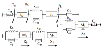Figure 4: The LMM of the recommended HMI platform

The LMM parameters in Figure 4 consists of screw shaft rotary inertia J_S, base massM_B, motor inertia J_M, screw shaft side equivalent mass M_S, handle mass M_T, equivalent torsional rigidity k_rot, ball screw nut rigidity k_n, axial base rigidity k_B, equivalent axial rigidity k_ax, DC motor torsional damping C_M, equivalent rotational damping C_rot, sides screw shaft damping C_S, ball screw nut damping C_n, axial guide damping C_g, axial base damping C_B, and equivalent axial damping C_ax.
Parameters (DOF) of the model shown in Figure 4 include,
θ_M- Angular rotation of the DC motor
θ_S- Angular rotation of screw shaft at handle position
X_B- Axial base displacement
X_S- Axial displacement of the screw shaft at handle position
X_T- Operating handle position
Equation 2 represents the mathematical model of a DC motor,

where, K_t and K_bm denote motor torque and back emf constants, L_ais winding leakage inductance, θ ̇_M is the angular velocity of the rotor inside motor, E_a is the voltage source, and R_a is the armature resistance. References [1,36] provide a detailed step by step Lagrange and state-space mathematical modelling for the physical structure in Figure 4.
Lagrange Model
Second order Lagrange’s equations are employed to develop the ball screw feed drive system’s dynamic model. Lagrange function is defined by the variation between kinetic and potential energies of a physical system. Equation (3) gives the mathematical relations for total kinetic energy (T), potential energy (U) and dissipation function (D), associated with the total system.

Equation (5) represents the Lagrangian function of a system. This function is calculated about force ‘Q’ and the generalized coordinate ‘q’.

Coordinates ‘q’ and ‘Q’ indicate independent coordinates and force inputs to the physical system respectively, given by the following relations in (6),

On solving (4) using (5) and (6), the following set of equations were obtained,

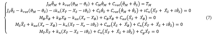
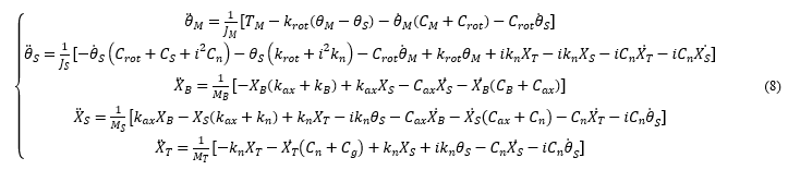
After rearranging the terms in (7), a set of five equations are obtained, that is given in (8). Based on these equations, the Simulink model is built on the MATLAB software, this software-based mathematical model is displayed in Figure 5.

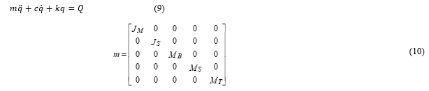
LMM of the proposed design, is given in matrix form by the following relation in (9),
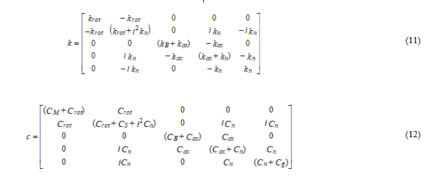
Equations (10), (11) and (12) indicate the values for matrices m, k and c respectively. These matrix values are acquired from (7).

State-Space Model and Transfer Function
Matric values given in (10-12), are substituted in (13), to provide the state-space representation of system model.

For the state-space model, we first determine the number of states. In this experiment, each of the five equations in (7) are second-order differential equations, i.e, each equation will include at least two states.
State-state model is represented as, x ̇=Ax+Bu and y=Cx+Du. In this system A is (11×11) matrix, B is (11×1) matrix, C is (1×11) matrix and D matrix is 0.
Equations (14) and (15) represent the State- space model and Transfer function of the system.

where X=[ x_1 x_2… x_11 ].The output is the operating handle position (X_T ), which is assigned to the state variable x_10.
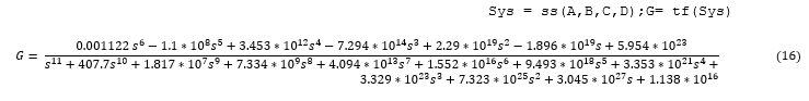
The transfer function (G) stated in (16) is obtained from the state-space model by using the following MATLAB codes,
Sys = ss(A,B,C,D);G= tf(Sys)

The Controllability and Observability of the system can be obtained from its state- space model in (14). The Controllability matrix (C_M) and Observability matrix (O_M) were calculated using the following MATLAB commands, ‘ctrb(A,B)’ and ‘obsv(A,C)’ respectively. Both the matrices were found to be invertible with their determinant values not equal to zero. Thus, this shows that the system is controllable and observable.

Figure 5: Simulink Block of the concerned Haptic Machine Interface (hardware platform)

Algorithm and Simulink Modelling of ADRC
ADRC originates from the classical PID controller, retaining the central idea of error feedback control. The drawbacks of the PID controller are overcome by the significant dynamic structure of ADRC. As seen in Figure 6, an ADRC architecture is composed of three parts, namely, the Tracking Differentiator (TD), Extended State Observer (ESO) and Nonlinear State Error Feedback (NLSEF). Each of the subsystems is explained here, followed by their Simulink model created on MATLAB.

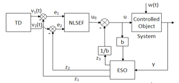Figure 6: Basic ADRC structure of a two- order system

 

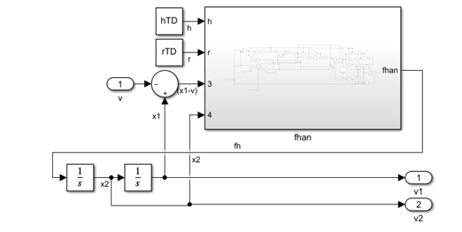Figure 7: Simulink Model of TD subsystem

Definitions of parameters used for ADRC design: v_1 (t) or v_1 is the tracking signal, and v_2 (t) or v_2is the differential signal of the given input signal. The output signal of the system and input signal of ESO is given by ‘y’. u is called the control volume, it is the input signal of the controlled object and the ESO. z_1and z_2are variables of the estimated state. z_3is the estimated signal of the total disturbance, i.e., both internal disturbance and the external interference present. w(t) is the external disturbance acting on the concerned system. e_1and e_2 are the error signals fed to the NLSEF.
Tracking Differentiator (TD)
TD determines the transition process for the system input, in order to obtain a smooth input signal v_1 (t) which is the desired trajectory and its differential signal v_2 (t). Consider the input signal v(t) is to be differentiated, thus, TD provides the fastest tracking v(t) given by (18). By solving the following differential equation, the required transient profile is obtained.

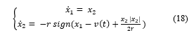
The parameter r is chosen according to the speed of the transient profile, i.e., to expedite or moderately slow down the transient profile. v is the desired value for x_1. The Simulink model of TD is shown in Figure 7, wherein fhan is a nonlinear function denoted as fhan(x_1-v,x_2,r,h). h is the simulation step, also called the sampling period.

The function fhan is presented later in this paper. Equation (19) is a time-optimal solution provides no overshoot and fastest convergence from v_1 to v. Parameters r_0 and h_0 are equated to r and h respectively [10].

Nonlinear State Error Feedback (NLSEF)

The control law of PID controller implements a linear combination of the present, past and future predictive kinds of the tracking error. For an infinite time, the tracking error attains zero value for linear feedback systems. Whereas, for a nonlinear feedback function given in (20), the error can reach zero value much earlier in a finite time (α<1). Such a mechanism significantly alleviates the steady-state error in comparison to an integral control [10]. Thus, in an ADRC control framework, the nonlinear feedback functions fal and fhan play a significant role during operation.

The Simulink model of NLSEF seen in Figure 8, has been developed using the mathematical relations from (20-23).

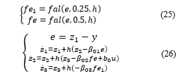
Parameter c denotes the damping coefficient. And function fhan(x_1,x_2,r,h) is represented using the following set of equations [37],

where,

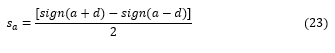
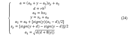
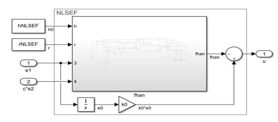Figure 8: Simulink Model of NLSEF subsystem

Extended State Observer (ESO)

ESO estimates full system states and the total effect of disturbances (or extended states) in real-time. These disturbances may arise from unknown or nonlinear system dynamics of the manipulator, external disturbances, and mismatch of control parameters. Thus, in robot control, ESO present in the feedback loop is used to estimate and cancel the effects of these uncertainties. Figure 9 gives a detailed Simulink model of the ESO block. This subsystem constitutes of the nonlinear feedback function fal defined in (20). The algorithm for ESO is characterized as follows [37,38]:

where, β_01,β_02,β_03 are parameters of ADRC that can be obtained from the system’s sampling step. Thus, four main parameters to be controlled are, simulation step (h), control gain (r), damping coefficient (c) and compensation factor (b_0).

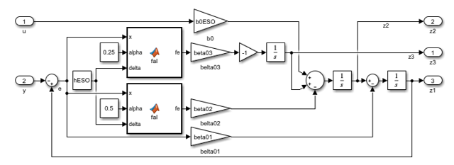Figure 9: Simulation Model of ESO subsystem

Figure 10: Simulink model of ADRC system including the HMI as the Controlled object

Controlled Object

The integration of TD structure, with the NLSEF structure, followed by the nonlinear ESO structure (which provides total disturbances estimation and rejection), altogether constitute the ADRC system. This controller is integrated with the HMI system. The Simulink model of HMI shown in Figure 5, is called the Controlled object in the ADRC system as seen in Figure 10.

Results and Discussions

Validation of the consistence between the physical interface system and the Simulink model
Figure 11 depicts the output response of the proposed physical system with PI controller, and Figure 12 depicts the LMM’s response executed via MATLAB and Simulink.

Figure 11: Output response of handle position from the physical system

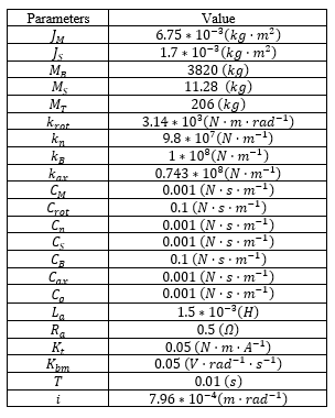
As seen in Figures 11 and 12, except for the magnitude, output response curves obtained from the physical interface platform and from the Simulink model respectively, are found to be similar. Dissimilarity in magnitude is mainly because, firstly, the units of the Y-coordinates are distinct. Secondly, it is difficult to measure the lumped parameter values of the physical platform. Thus, the proposed platform’s parameter values are slightly different from the simulation model values (i.e. designed via Simulink). Yet the simulation model substantiated the fundamental characteristic of the recommended HMI platform. The parameter values that were used in the Simulink model are listed in Table 1.

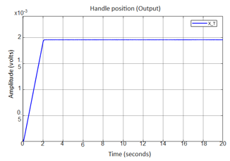Figure 12: Output response of the Handle position (X_T) from Simulink model

Table 1: Parameter values of HMI used in Simulink Model

5.2. Disturbance rejection performance of the designed ADRC controller and comparison with PI controller

Experimental analysis of the comparison between ADRC and PI controllers is based on the following performance indices, that is, the system response obtained in the vicinity of disturbance present in the motor voltage, and controller variable values of both the controllers. The volatage unstability in the motor is one of the primary disturbance to the control system. In this experiment, the disturbance on the voltage supply to the motor is added to validate the disturbance rejection performance of the designed ADRC and PI controllers. The disturbance is added at the 5th second with an amplitude of 5000mV and lasting 0.2s, as shown in Figure 13.
Figure 14 shows the system response of the system controlled by ADRC and PI controllers. For the sake of fair comparison, the ADRC and PI controllers are tuned to have similar overshoot values. From Figure 14, one can find the system response with ADRC (Figure 14(a)) goes back to the reference value quickly after the overshot, however, the PI controller takes longer time to do so. Both system responses are affected by the disburance (starting from 5s in Figure 14), but the ADRC controlled system gets much smaller shift from the reference value than the PI controller.
Figure 15 demonstrates the control variable values of the two controllers, which depicts more details on controller behaviour. From Figure 15(a), one finds the ADRC controller starts with a mild control at the beginning due to the soften effect obtained in the tracking differentiator, which makes a smaller peak value on the control (Figure 15(a)). When the disturbance happens, the designed ADRC depresses the shift from reference value greatly, which leads to only a small change on the system response (refer to Figure 15(a)) from 5s. The PI controller is much more rigid when compared with the designed ADRC, which makes the controller start with an aggressive control (Figure 15(b)) at the beginning, and bigger shift from the reference value after the disturbance (refer to Figure 15(b)) from 5s.
These advantages of the system response controlled by ADRC can be explained in Figure 16, i.e. the total disturbances estimated by the ADRC. From Figure 16, one finds at the beginning of the control, the intial stage of the input step signal is considered as a disturbance (around 0s in Figure 16) which is compensated to obtain a soft rise of the system. This is obtained by the TD. When the disturbance occurs (around 5s in Figure 16), it is considered as disturbance (z3 in (26)) as well and is compensated accordingly. Now the ESO observes the disturbance, and is compensated to the control variable generated by the NLSEF. This mechanism is shown in Figure 10. Thus, this disturbance rejection property of ADRC controller makes it unique in operation as compared to the PI controller.

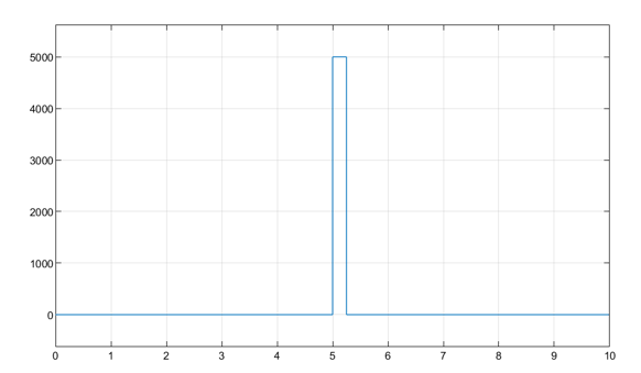Figure 13: The added voltage disturbance in motor

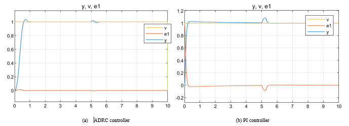Figure 14: System response

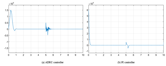Figure 15: Control variable values

Figure 16: Estimated total disturbances by the ADRC

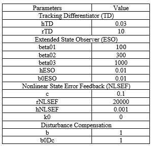
Table 2: Parameter values of the ADRC system

Conclusions and Future work

The shift of feedback control paradigm design has been extensively studied over the past few decades. With a huge potential of disturbance rejection control method, this paradigm shift will play a critical role in the migration from the primitive PID controller to an ADRC. A PID controller passively responds to disturbances, causing zone oscillations. But on the other hand, ADRC actively rejects disturbances, delivering a smooth control system. In an ADRC, the unmeasurable states and total disturbances are actively compensated by the ESO present in the feedback loop. Whereas TD effectively acquire the continuous and differential form of signals from a measurement signal containing random noise, or from a discontinuous signal. It is easy to tune the parameters of TD due to its model independence property. The nonlinear feedback combination (NLSEF) of the two nonlinear functions play a significant role in this recently proposed control framework. Thus, considering the system parameters and model uncertainties, ADRC shows higher tolerance with merits of simple and intuitive model-free control design methods. Along with, it needs less energy in control in comparison to other control strategies.
This paper gives a detailed step by step design and mathematical modelling of the proposed HMI system developed for the research. After installation of the mechanical and electrical hardware components, Lagrange equations were derived based on the LMM of the system. An ADRC controller was designed and integrated with the haptic display platform Simulink model. Simulation studies were conducted to illustrate the efficiency and robustness of the ADRC controller.
However, up to date, debates and inconsistencies on the new paradigm concept still exist, and reports and validation on the successful integration of ADRC into the field of control theory are quite limited. This work pushes the realms of ADRC integration with actual physical plants for practical applications, and potentially opens up new realms constituting of new control laws formulated through experimentation.
Future research of this project will include the analysis of ADRC controller for a two-axis ball screw driving system dealing with time delay, and coupling between the two axes of the experiment. This analysis will be conducted with the modelling environment created on MATLAB/ Simulink.

Conflict of Interest

The authors declare no conflict of interest.

Acknowledgment

The financial assistance of the National Research Foundation (NRF) towards this research is hereby acknowledged. Opinions expressed and conclusions arrived at, are those of the author and are not necessarily to be attributed to the NRF.

1. S.N.F. Nahri, S. Du, B. Van Wyk, “Haptic System Interface Design and Modelling for Bilateral Teleoperation Systems,” in 2020 International SAUPEC/RobMech/PRASA Conference, IEEE: 1–6, 2020, doi:10.1109/SAUPEC/RobMech/PRASA48453.2020.9041010.
2. K. Abidi, Y. Yildiz, B.E. Korpe, “Explicit time-delay compensation in teleoperation: An adaptive control approach,” International Journal of Robust and Nonlinear Control, 26(15), 3388–3403, 2016, doi:10.1002/rnc.3513.
3. P.F. Hokayem, M.W. Spong, “Bilateral teleoperation: An historical survey,” Automatica, 42(12), 2035–2057, 2006, doi:10.1016/j.automatica.2006.06.027.
4. D.S. Nunes, P. Zhang, J. Sa Silva, “A Survey on Human-in-the-Loop Applications Towards an Internet of All,” IEEE Communications Surveys & Tutorials, 17(2), 944–965, 2015, doi:10.1109/COMST.2015.2398816.
5. D.A. Lawrence, “Stability and transparency in bilateral teleoperation,” IEEE Transactions on Robotics and Automation, 9(5), 624–637, 1993, doi:10.1109/70.258054.
6. L.Y. Ang K, Chong G, “PID control system analysis, design, and technology,” IEEE Transactions on Control Systems Technology, 13(4), 559–576, 2005, doi:10.1109/tcst.2005.847331.
7. D. Sun, F. Naghdy, H. Du, “Wave-Variable-Based Passivity Control of Four-Channel Nonlinear Bilateral Teleoperation System Under Time Delays,” IEEE/ASME Transactions on Mechatronics, 21(1), 238–253, 2016, doi:10.1109/TMECH.2015.2442586.
8. E. Nuño, L. Basañez, R. Ortega, “Passivity-based control for bilateral teleoperation: A tutorial,” Automatica, 47(3), 485–495, 2011, doi:10.1016/j.automatica.2011.01.004.
9. A. Gupta, M. Kilchenman, O.’ Malley, M.K. O’malley, “Disturbance-Observer-Based Force Estimation for Haptic Feedback MRI-compatible robotics View project Haptic Paddle View project Disturbance-Observer-Based Force Estimation for Haptic Feedback,” Article in Journal of Dynamic Systems Measurement and Control, 133(1), 2011, doi:10.1115/1.4001274.
10. J. Han, “From PID to Active Disturbance Rejection Control,” IEEE Transactions on Industrial Electronics, 56(3), 900–906, 2009, doi:10.1109/TIE.2008.2011621.
11. Z. Gao, “Active disturbance rejection control: a paradigm shift in feedback control system design,” in 2006 American Control Conference, IEEE: 7 pp., 2006, doi:10.1109/ACC.2006.1656579.
12. Y. Huang, W. Xue, “Active disturbance rejection control: Methodology and theoretical analysis,” Elsevier, 53(4), 963–976, 2010, doi:10.1016/j.isatra.2014.03.003.
13. H. Feng, B.-Z. Guo, “Active disturbance rejection control: Old and new results,” Annual Reviews in Control, 6, 1–11, 2017, doi:10.1016/j.arcontrol.2017.05.003.
14. H. Jin, W. Lan, Y. Chen, “Replacing PI Control With First-Order Linear ADRC,” in 2019 IEEE 8th Data Driven Control and Learning Systems Conference (DDCLS), IEEE: 1097–1101, 2019, doi:10.1109/DDCLS.2019.8908981.
15. J. Han, “A class of extended state observers for uncertain systems,” Control and Decision, 10, 85–88, 1995.
16. J.Q. Han, “Auto Disturbance Rejection Controller and It’s Applications,” Control and Decision, 13, 19–23, 1998, doi:NII Article ID (NAID) 10007201534.
17. Zhiqiang Gao, Yi Huang, Jingqing Han, “An alternative paradigm for control system design,” in Proceedings of the 40th IEEE Conference on Decision and Control (Cat. No.01CH37228), IEEE: 4578–4585, 2001, doi:10.1109/CDC.2001.980926.
18. Z. Gao, “On the centrality of disturbance rejection in automatic control,” ISA Trans, 53(4), 850–857, 2014, doi:10.1016/j.isatra.2013.09.012.
19. Q. Zheng and Z. Gao, “On practical applications of active disturbance rejection control,” in Proceedings of the 29th Chinese control conference, 6095–6100, 2010, doi:INSPEC Accession Number: 11572423.
20. G. Herbst, “A Simulative Study on Active Disturbance Rejection Control (ADRC) as a Control Tool for Practitioners,” Mdpi.Com, 2(4), 246–279, 2013, doi:10.3390/electronics2030246.
21. A. Ortiz, S. Orozco, I. Zannatha, “ADRC controller for weightlifter Humanoid robot,” in 2019 International Conference on Electronics, Communications and Computers (CONIELECOMP), IEEE: 41–46, 2019, doi:10.1109/CONIELECOMP.2019.8673147.
22. Z.Q. W. Chenlu, C. Zengqiang, S. Qinglin, “Design of PID and ADRC based quadrotor helicopter control system,” in 2016 Chinese Control and Decision Conference (CCDC), 5860–5865, 2016, doi:https://doi.org/10.1109/CCDC.2016.7532046.
23. W.T. C. Fu, “Tuning of linear ADRC with known plant information,” ISA Trans, 65, 384–393, 2016, doi:doi:10.1109/access.2018.2805782.
24. Z. Chen, Q. Zheng, Z. Gao, “Active Disturbance Rejection Control of Chemical Processes,” in 2007 IEEE International Conference on Control Applications, IEEE: 855–861, 2007, doi:10.1109/CCA.2007.4389340.
25. G. Niemeyer, J.-J.E. Slotine, “Stable adaptive teleoperation,” IEEE Journal of Oceanic Engineering, 16(1), 152–162, 1991, doi:10.1109/48.64895.
26. Z. Chen, F. Huang, W. Sun, W. Song, “An Improved Wave-Variable Based Four-Channel Control Design in Bilateral Teleoperation System for Time-Delay Compensation,” IEEE Access, 6, 12848–12857, 2018, doi:10.1109/ACCESS.2018.2805782.
27. C.P. J. H. Ryu, J. Artigas, “A passive bilateral control scheme for a teleoperator with time-varying communication delay,” Mechatronics, 20, 812–823, 2010, doi:doi:10.1016/j.mechatronics.2010.07.006.
28. L. Sheng, U. Ahmad, Y. Ye, Y.-J. Pan, “A Time Domain Passivity Control Scheme for Bilateral Teleoperation,” Electronics Mdpi.Com, 8(3), 325, 2019, doi:10.3390/electronics8030325.
29. X. Xu, B. Cizmeci, C. Schuwerk, E. Steinbach, “Model-Mediated Teleoperation: Toward Stable and Transparent Teleoperation Systems,” IEEE Access, 4, 425–449, 2016, doi:10.1109/ACCESS.2016.2517926.
30. E.J. RodrIguez-Seda, Dongjun Lee, M.W. Spong, “Experimental Comparison Study of Control Architectures for Bilateral Teleoperators,” IEEE Transactions on Robotics, 25(6), 1304–1318, 2009, doi:10.1109/TRO.2009.2032964.
31. S. Hirche, M. Buss, “Human-Oriented Control for Haptic Teleoperation,” Proceedings of the IEEE, 100(3), 623–647, 2012, doi:10.1109/JPROC.2011.2175150.
32. L. Zhao, L. Liu, Y. Wang, H. Yang, “Active Disturbance Rejection Control for Teleoperation Systems with Actuator Saturation,” Asian Journal of Control, 21(2), 702–713, 2019, doi:10.1002/asjc.1767.
33. Q. Wang, M. Ran, C. Dong, “On Finite-Time Stabilization of Active Disturbance Rejection Control for Uncertain Nonlinear Systems,” Asian Journal of Control, 20(1), 415–424, 2018, doi:10.1002/asjc.1558.
34. C. Zhang, J. Yang, S. Li, N. Yang, C. Zhang, N. Yang, J. Yang, S. Li, “A generalized active disturbance rejection control method for nonlinear uncertain systems subject to additive disturbance,” Nonlinear Dynamics, 83(4), 2361–2372, 2016, doi:10.1007/s11071-015-2487-1.
35. S. Frey, A. Dadalau, A. Verl, “Expedient modeling of ball screw feed drives,” Producition Engineering, 6(2), 205–211, 2012, doi:10.1007/s11740-012-0371-0.
36. L. Luo, W. Zhang, Electromechanical Co-Simulation for Ball Screw Feed Drive System, IntechOpen, 2019, doi:10.5772/intechopen.80716.
37. Y.D. YV Wen-bin, “Modeling and Simulation of an Active Disturbance Rejection Controller Based on Matlab/Simulink,” International Journal of Research in Engineering and Science (IJRES), 3(7), 62–69, 2015, doi:www.ijres.org.
38. Z. Gao, Q. Zheng, L.Q. Gao, “On Validation of Extended State Observer Through Analysis and Experimentation ADRC: a new paradigm of the science of automatic control View project ADRC: Problem Solving View project On Validation of Extended State Observer Through Analysis and Experimentation,” Article in Journal of Dynamic Systems Measurement and Control, 134(2), 2012, doi:10.1115/1.4005364.

(Click Here)