1. V. Miglietta, M. Dhanak, “Current turbine array placement in quasigeosterophic flows over bottom topography,” in Oceans Conference, Seattle, WA, USA, 2019.
2. E. Johnson, “Quasigeostrophic flow over isolated elongated topography,” Deep-Sea Research, 29(9A), 1085-1097, Pergamon Press Ltd., Great Britain, 1982.
3. C. Garrett, P Cummins, “The efficiency of a turbine in a tidal channel,” Journal of Fluid Mechanics, 588, 243–251, 2007, doi:10.1017/S0022112007007781.
4. R. Vennell, “Tuning turbines in a tidal channel,” Journal of Fluid Mechanics, 663, 253-267, 2010, doi:10.1017/S0022112010003502
5. R. Vennell, “Realizing the potential of tidal currents and the efficiency of turbine farms in a channel,” Renewable Energy, 47, 95-102, Elsevier, 2012, doi: https://doi.org/10.1016/j.renene.2012.03.036
6. C. Christian, R. Vennel, “Efficiency of tidal turbine farms,” Coastal Engineering Proceedings, 1(33), structures.4, 2012, doi:https://doi.org/10.9753/icce.v33.structures.4
7. S. Draper, T. Nishino, “Centered and staggered arrangements of tidal turbines,” Journal of Fluid Mechanics, 739, 72-93, Cambridge University Press, 2014, doi:10.1017/jfm.2013.593
8. G. Carter and M. Gregg and M. Merrifield. “Flow and mixing around a small seamount on Kaena Ridge, Hawaii,” Journal of Physical Oceanography, 36, 1036-1052, 2006.
9. R.E. Brainard, “Fisheries aspects of seamounts and Taylor columns,” Master’s Thesis, Naval Postgraduate School. Monterey, California, 1986.
10. W. Owens and N. Hogg. “Oceanic observations of stratified Taylor columns near a bump,” Deep-Sea Research, 27A, 1029-1045, Pergamon Press Ltd., Great Britain, 1979.
11. A. Rogers, The biology of seamounts:25 years on., vol 79, Advances in marine biology, 2018. Doi 10.1016/bs.amb.2018.06.001
12. G.I. Taylor, “Motion of solids in fluids when the flow is not irrotational,” Proc. Royal Society of London, Series A, Containing papers of a mathematical and physical character, 93, 99-113, 1917.
13. M. Buckley, “Taylor Columns,” Course website for weather and climate laboratory at the Massachusetts Institute of Technology, 2004, Accessed June 2015. http://paoc.mit.edu/12307/reports/tcolumns.pdf
14. J.W.M. Bush, H.A. Stone, J.P. Tanzosh, “Particle motion in rotating viscous fluids: Historical survey and recent developments,” Current Topics in The Physics of Fluids, 1, 337-355, 1994.
15. J. Clarke, Andrew Grant, Gary Connor, C.M. Johnstone, “Development and in sea performance testing of a single point mooring supported contra-rotating tidal turbine,” in ASME 28th International Conference on Ocean Offshore and Arctic Engineering, 2009, doi:10.1115/OMAE2009-79995.
16. R. Hide, “Origin of Jupiter’s Great Red Spot.” Nature, 190, 895-896, 1961.
17. P.J. Mason, R.I. Sykes, “A numerical study of rapidly rotating flow over surface-mounted obstacles,” Journal of Fluid Mechanics, 111, 175-195. Great Britain, 1981.

(Click Here)

(Click Here)

1.Introduction

Special considerations for large underwater turbine farms or arrays at mid and high latitudes will be necessary because at such latitudes the Coriolis force can measurably impact the dynamics of flow in asymmetric patterns.  A thoughtful and robust array design can position turbines to harness the Coriolis force[1].  Array design requires knowledge of the local dynamics and an understanding of all forces including the Coriolis force. Tools for evaluating such an ocean engineering endeavor includes numerical solutions for flows moving past extended obstacles in instances when rotational forces are required to describe the flow [2].

The Coriolis force is a pseudo force caused by Earth spinning on its axis. Typical ocean engineering problems ignore Coriolis effects because they are minimal on the typical scale of ocean engineering problems. Also, local inertial forces often dominate engineering problems where a good approximation allows for the Coriolis force to drop out of consideration.  But for tidal currents, the local inertial speeds will drop to zero at least twice daily, and it is at these periods where the Coriolis force may impact an array.  A renewable energy system’s array which produces electricity for a municipal power grid will be sensitive to electrical and therefore environmental energy fluctuations. For locations with higher values of latitude the Coriolis force should be considered at periods surrounding slack tide.

Often tidal current power sites are limited to channels and bays [3-7], however tides are not limited to these locations.  Tides occur throughout the Earth’s oceans.  Here the design of a turbine array in open water is analyzed. Vertical boundaries are far from the array and the domain’s distinct boundaries are the surface of the water and the seafloor.  A very long array, capable of being economically viable, composed of a single line of turbines is considered.  The turbine array is taken to be 10,000m long. The large dimension is comparable to a topographic feature and certainly would allow for the array to meet a production goal on the order of megawatts of electricity.  It is hypothesized that a very large array in the ocean would experience the same amplification of flow rate around it that a seamount experiences [8, 9].

Studies of seamounts, and underwater ridges indicate flow behavior around large obstructions in the ocean are influenced in a measurable way by the Coriolis force [2, 8, 10].  The largest dimension of 10,000m would put a turbine array on the scale of a small seamount and on par with the scale of a seamount [10].  It has been observed that flows past/around seamounts are amplified and that the flow above them is best described as stagnant [10].  These are rotational effects and have been of interest to marine biologists and oceanographers [9, 11].

The flow patterns and Coriolis effects on an underwater turbine array differ from those of wind turbine arrays because of the huge density difference between air and water.  The nature of air and water differ in a way where the rotational phenomenon of Taylor columns are not found in the atmosphere for quasigeostrophic flow conditions [12, 13].  These Coriolis effects are not seen around wind farms or wind turbines because they disappear in a density gradient.

2. Background

2.1. Not a channel

Studies like [4-6] look at tidal channels being utilized for tidal current power.  However, taking over an entire tidal channel or even a good portion of one for power generation would have serious consequences for the established use of a channel. Many channels have daily uses which include maritime traffic for shipping, fishing and recreation. Obtaining permits and backing of local communities to re-purpose heavily used tidal channels for power production would likely be a challenge. If the tidal power project was for a remote community or some remote operations then challenges could be different.  However, for large coastal communities looking to harness tidal power across a tidal channel such challenges could be expected. For example, the offshore wind development off the coast of Massachusetts, Vineyard Wind, has experienced a lot of push back by the fishing industry in the area.  The project has been on hold since 2019 while the Interior Department conducts a review.  Harnessing tidal current power in more open areas, could be less oppressive to current users of waterways.  In this study the ideal deployment area is far from boundaries like shorelines, piers, or breakwaters.

2.2. Static Obstruction in a Rotational Fluid

Here the effects of the static physical presence of an obstruction to flow in a changing tide were studied.  The review of studies of the effects of seamounts on the flow around them shows that large obstructions, like that which could be expected from a tidal turbine array, produce asymmetric patterns seen in rotational fluids [14]. These rotational effects are caused by the spinning of the Earth. The fundamental physical dynamics for an obstruction to flow in a rotational fluid with a small inertial current is similar for a bottom seated obstruction and an obstruction suspended in the water column [14]. An array would have similar effects for both bottom seated and moored or suspended turbines in the water column.

Furthermore, the research presented here would be applicable to the tidal array design engineering as well as the deployment site assessment. The physical phenomenon of Taylor columns and their associated flow patterns could develop locally at the site of the engineered structure itself, and it could also develop on/around a bathymetric feature like a ridge or seamount where an array or turbine is deployed. The University of Strathclyde encountered what was described as a spatial-temporal eddy with a ‘calm’ center when it was testing a tidal current turbine [15]. This could have been caused by a Taylor column which has a stagnant interior.  The latitude for their deployment was approximately 55N.

2.3. Unchanging Coriolis Parameter in the f-plane

This study evaluates an array so large it can be viewed at the scale of topography, i.e. the array will define the ‘landscape’ in the area it is deployed. The f-plane approximation is made, where the Coriolis parameter does not change. If the array was to extend over several degrees of latitude the Coriolis parameter would change and a structure so great in size would need to be analyzed in the β-plane. For the f-plane approximation, the absolute velocity of the tidal current will be the parameter that changes the blocking parameter cyclically over time i.e. with the tidal cycle.

2.4. Blocking Parameter

The blocking parameter correlates the size of the obstruction with environmental parameters to indicate the degree of influence the structure has on the local flow patterns. A critical blocking parameter predicts the formation of a Taylor column. A Taylor column is a hydrodynamic phenomenon, parallel to the axis of rotation, which appears like an extension of an object, obstructing flow when the blocking parameter is at a critical value. The critical value of the blocking parameter S, is O(1).  There is no consensus on a more exact value for the blocking parameter.  For the [10] observations the blocking parameter appeared to be approximately 0.7. The exact blocking parameter is likely to be site specific and will vary on a range of environmental parameters. Important parameters include the height of the array, h; the depth of the water, d, and the latitude which changes the Coriolis parameter, ?.

This study uses the definition of the blocking parameter by [16],

S = h/(d•R₀)

S = ?hL/(d•U)                                   (1)

There is no consensus on the calculation of the blocking parameter or its critical value. The formation of a Taylor column was initially linked to the Rossby number dropping below the value of  1/π  [12].  Effectively this original critical blocking parameter was when the Rossby number, R₀,was 1/π or smaller.

Further research [16] on rotational fluids added a coefficient to the inverse of the Rossby number,  the ratio of the height of  the obstruction to the depth of the water, h/d.  Decades later [17] used the ratio of the greatest horizontal length of the obstruction to the water depth as the coefficient to the inverse of the Rossby number. The similar thread in all these blocking parameters is the Rossby number.  The Rossby number is the ratio of inertial forces to rotational forces. The rotational forces are represented in the Rossby number by the terms ?L. Where L is the characteristic length, the longest horizontal dimension of the object. The Coriolis parameter is larger for higher latitudes. The Rossby number will decrease for higher latitudes because at these locations rotational forces are stronger. The Rossby number is inversely proportional to the Coriolis parameter

R₀ ∝1/?                                          (1)

and the blocking parameter is proportional to the Coriolis parameter

S∝?                                                (2)

Consequently, a structure located at a higher latitude will experience a higher blocking parameter; with velocity, and structure size, and water depth all remaining constant.

The Rossby number includes L, the characteristic length of an object.  The [16] blocking parameter is the most complete because it not only includes the characteristic length of an object, but it also includes its height.  The [17] blocking parameter is redundant in that it uses the length of the obstruction in its coefficient and the length also appears in the Rossby number. So effectively the [17] blocking parameter uses the square of the characteristic length. Returning to the perspective of a tidal current, the velocity will change and with it the blocking parameter will change. Recall that the blocking parameter is inversely proportional to the velocity

S ∝1/U                                           (3)

Looking at the critical blocking parameter for various latitudes, faster speeds can bring about a critical blocking parameter at higher latitudes. This means that the period of the tidal cycle where the blocking parameter is critical will be longer at higher latitudes.

3. Problem Statement

Since it is during the slack tide that the Coriolis force could impact the dynamics of a turbine array, this period cannot be passed over simply as the period where tidal current turbines will not produce electricity. At slack tide, the water is in quasigeostrophic flow; meaning that the inertial current is minimal and the Coriolis force is needed to describe the flow.  In quasigeostrophic flow, the consequence of a small inertial current is that it prevents the equilibrium of the pressure force and Coriolis force (this equilibrium is described as geostrophic flow).

During each tidal change the blocking parameter becomes critical.  The critical value of the blocking parameter is associated with the formation of a Taylor column.  When this happens the array (the obstruction) will behave like a taller structure, or it will have a sort of physical shadow above it (and possibly below it).  Also, for a critical blocking parameter the flow can be described well by a 2-D approximation, where the velocity does not vary in the water column. This flow described by the 2-D approximation, i.e. a Taylor column, can appear almost instantaneously in a laboratory tank. The question addressed is what are the characteristics of the flow influenced by the Coriolis force in the immediate vicinity of a linear array?  The equipment in a tidal zone is likely to experience rotational effects during periods when currents change direction. Asymmetric flow for quasigeostrophic conditions have been observed around seamounts and in this study modelling was used to predict how a large linear array would experience such conditions.

3.1. Method

The blocking parameter, S, will have a spiked value at every tidal change because it is inversely proportional to the velocity. Numerical [2] solutions were used to plot the velocity around a linear array when the blocking parameter was critical or O(1). The solutions depend on the angle of the incident flow, α, and also depend on the ratio, γ,  of the largest dimension, L, to the smallest dimension, l,  in the X-Y plane.

γ = L/l                                          (4)

The solution is insensitive to the details of the shape of the obstacle [2]. Solutions model flow patterns closely to those in the oceans where the bathymetry is more complex than a simple ellipse [2]. The solution is for a homogeneous, inviscid, incompressible flow, with a constant depth, in a rotating frame, and it satisfies the conservation of potential vorticity.  The stream function used [2] in elliptical coordinates (μ, θ) is:

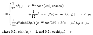4. Results

An idealized smooth diurnal tide, with equal peaks is considered for analysis. The far field velocity, U, changes the blocking parameter, S, as the tidal velocity changes. The height, h, is taken to be 10m, and the water depth, d, to be 35m. Aspect ratios between 1,000 and 250 do not vary the results remarkably. For steady quasigeostrophic flow the streamlines do not vary in the Z direction as long as there is no density gradient.  The results show that directly at, or adjacent to, the structure is where the system could be impacted by the unique dynamics of periods dominated by quasigeostrophic flow. The character of the rotational effects is asymmetric and for the linear array placed in quasigeostrophic incident flow, the flow around it is distinctly asymmetrical when modelled with [2] analytical solutions. The results for different blocking parameters were considered as “snapshots” of what may occur over time because the time variability of these processes is not understood. The velocity fields at both ends of an array placed perpendicular to the quasi-geostrophic flow were examined for a number of velocities/blocking parameters and plotted against time. The plots reveal that the accelerations on the left-hand side looking downstream were greater than the decelerations on the opposite side, Figure 1.  The corresponding effect on power over the period of quasi-geostrophic flow may be estimated from a plot of velocity cubed against time, Figure 2. The flow adjacent to the structure is most affected by the Coriolis force.

For such a perpendicular array (Figures 3 and 4) the flow is accelerated by a factor of 2 on one end, while on the opposite end it the flow rate is 1/2  to 1/5 of the far field velocity. The velocity coefficients at the end points do not change significantly as the blocking parameter increases.  For blocking parameters larger than one, the location of the minimal flow (i.e.  smallest velocity coefficient) moves away from the structure.  The location of the most accelerated flow does not move away from the structure in the same manner. When the blocking parameter increases, flow adjacent to a greater area of the structure experiences acceleration. Furthermore, there is a steady decrease in velocity across the perpendicular array for critical blocking parameters of O(1).

For an array placed  parallel to the quasi-geostrophic flow (Figures 5 and 6) the velocity gradient is very sharp over the array.  It is remarkable that for such a parallel array, the location of greatest flow deceleration moves significantly farther from the structure when the blocking parameter increases.  The sharp velocity gradient appears unrealistic and indicates occurrence of flow separation and high turbulence.

Figure 1: Graph of the idealized far field tidal velocity U and the different velocities at both ends of a linear array aligned perpendicular to the tidal velocity. Solutions for perpendicular flow and γ = 1,000

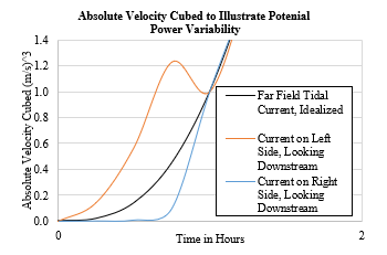Figure 2: The power produced from an ocean current is proportional to the velocity cubed.  A change in the flow around the structure during a tidal change may be experienced by sensitive power generation systems.

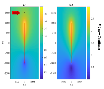Figure 3: Modeled flow velocity change factors are plotted in color for flow at the depth of the array during quasigeostrophic flow with a blocking parameter, S,  equal to 1 and 2. Flow direction is from the left to the right. The coordinate system is normalized using l, the minor axis of the elliptical body, which is 10m for the proposed array. The major axis L is 10,000m.  A velocity coefficient of 1 corresponds to the far field velocity U.

Figure 4: Modeled flow velocity coefficients are plotted in color for flow at the depth of the array during quasigeostrophic flow with a blocking parameter equal to 2.  A reduced velocity will increase the blocking parameter. The decelerated flow has moved away from the obstruction, as compared with S=1.  More of the flow adjacent to the obstruction has a velocity coefficient >1 when compared with S=1. Flow direction is from the left to the right. The coordinate system is normalized using l, the minor axis of the elliptical body.

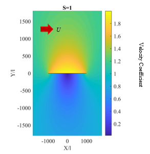Figure 5: The asymmetry of the flow is striking for an array oriented perpendicular to the current.  The area adjacent to the array has the greatest change in flow velocity. The array is modeled as static. Flow past the array has a blocking parameter, S = 1.  The far field velocity has a velocity coefficient of one. The coordinate system is normalized using l, the minor axis of the elliptical body.

Figure 6: Flow past the array during quasigeostrophic flow with a blocking parameter, S = 2.  The darkest blue point is the minimum velocity in the vicinity of the structure and this point has moved a significant distance, approximately half the characteristic length, L, away from the structure.

4.1. Design Plan

For a line of tidal current turbines at mid to high latitudes rotational flow effects caused by the Coriolis force can impact local dynamics at periods with small inertial currents.  The strongest changes in flow dynamics can occur directly adjacent to a structure obstructing a quasigeostrophic flow. Flow acceleration and deceleration can occur around the structure asymmetrically. It appears prudent to make the following design considerations:

• ensure that the linear array is placed perpendicular to the flow;
• review local tidal current data and decide if both ebb and flood currents, or just one direction, will be used for power production;
• prepare your system for an asymmetric velocity gradient, down the line of the array, at periods of tidal change.

One design recommendation for a site where both ebb and tide are utilized for energy production would be to separate the array into a minor and a major field with the two fields separated by supporting equipment. The major field placed on the left side of the array (looking downstream), for the strongest tidal direction.  Dummy turbines could be included in the central field of supporting equipment to elongate the array if the asymmetric flow pattern is especially desirable for a production location.

An array parallel to the incident flow is not recommended because of the sharp velocity gradient modeled over it for quasi-geostrophic flow. The modeled gradient is not realistic and suggests occurrence of flow separation and high turbulence.

5. Final Comments

Site specific investigations are crucial for effective array design and deployment.  All sites will have unique bathymetry and unique local currents.  The variables affecting the layout of the array will include the angle of incident flow; the aspect ratio of the array; the water depth and height of the array; and the latitude at which the array is placed. Placement at higher latitudes will produce higher blocking parameters. The Taylor column phenomenon can be produced by an engineered structure, bottom seated or suspended in the ocean, or by a larger bathymetrical feature on which an engineered structure is placed.

Conflict of Interest

The authors declare no conflict of interest.

Acknowledgment

A special thanks to the Department of Ocean and Mechanical Engineering at Florida Atlantic University.