1. I. Valieva, M. Björkman, J. Åkerberg, M. Ekström, I. Voitenko, “Multiple Machine Learning Algorithms Comparison for Modulation Type Classification for Efficient Cognitive Radio,” in MILCOM 2019 – 2019 IEEE Military Communications Conference (MILCOM), 318–323, 2019, doi:10.1109/MILCOM47813.2019.9020735.
2. D. Rosker, D. M., “DARPA Spectrum Collaboration Challenge (SC2).,” DARPA Spectrum Collaboration Challenge (SC2), 2020.
3. C. Xin, Spectrum Sharing for Wireless Communications, 2015.
4. O. Fink, Q. Wang, M. Svensén, P. Dersin, W.-J. Lee, M. Ducoffe, “Potential, challenges and future directions for deep learning in prognostics and health management applications,” Engineering Applications of Artificial Intelligence, 92, 103678, 2020, doi:https://doi.org/10.1016/j.engappai.2020.103678.
5. S. Peng, H. Jiang, H. Wang, H. Alwageed, Y.-D. Yao, “Modulation classification using convolutional Neural Network based deep learning model,” 1–5, 2017, doi:10.1109/WOCC.2017.7929000.
6. kaiyuan jiang, J. Zhang, H. Wu, A. Wang, Y. Iwahori, “A Novel Digital Modulation Recognition Algorithm Based on Deep Convolutional Neural Network,” Applied Sciences, 2020, doi:10.3390/app10031166.
7. Mathworks., Modulation Classification with Deep Learning., 2020.
8. M. Véstias, R. Duarte, J. Sousa, H. Neto, “Fast Convolutional Neural Networks in Low Density FPGAs Using Zero-Skipping and Weight Pruning,” Electronics, 8, 2019, doi:10.3390/electronics8111321.
9. Z. Zhu, Automatic Modulation Classification: Principles, Algorithms and Applications, John Wiley & Sons, Incorporated, 2015.
10. A. Kubankova, H. Atassi, A. Abilov, “Selection of optimal features for digital modulation recognition,” 2011.
11. W. Gardner, Cyclostationarity in Communications and Signal Processing, IEEE Press, New York, 1994.
12. W.A. Gardner, C.M. Spooner, “Cyclic spectral analysis for signal detection and modulation recognition,” in MILCOM 88, 21st Century Military Communications – What’s Possible?’. Conference record. Military Communications Conference, 419–424 vol.2, 1988, doi:10.1109/MILCOM.1988.13425.
13. C. Cormio, K.R. Chowdhury, “A survey on MAC protocols for cognitive radio networks,” Ad Hoc Networks, 7(7), 1315–1329, 2009, doi:https://doi.org/10.1016/j.adhoc.2009.01.002.
14. M. Raina, G. Aujla, “An Overview of Spectrum Sensing and its Techniques,” IOSR Journal of Computer Engineering, 16, 64–73, 2014, doi:10.9790/0661-16316473.
15. K. Hinkelmann, Design and analysis of experiments., John Wiley & Sons, Inc., 2011.
16. C. Rajan, Statistics for Scientists and Engineers, John Wiley & Sons, Incorporated, 2015.
17. Mathworks, Mean or median absolute deviation, 2020.
18. Mathworks, Root-mean-square level, 2020.
19. Mathworks, Zero Crossing Rate, Nov. 2020.
20. Mathworks, Interquartile range, 2020.
21. Mathworks, 75th Percentile, 2020.
22. Mathworks, Fading Channels, 2020.

(Click Here)

(Click Here)

1.Introduction

This paper is an extension of the work “Multiple Machine Learning Algorithms Comparison for Modulation Type Classification for Efficient Cognitive Radio” originally presented in Milcom 2019 [1].

The global market of mobile devices and services actively using the electromagnetic spectrum is continuously growing. Traditionally the electromagnetic spectrum utilization has been performed using a robust static approach developed almost a century ago: it rations access to the spectrum in exchange for the guarantee of interference-free communication spectrum is divided into the rigid, exclusively licensed bands, allocated over large, geographically defined regions. In conditions when some of these license bands are being nearly unused, while the others are overwhelmed, the problem of spectrum scarcity arises [2]. To cope with the increasingly populated spectrum, the electromagnetic spectrum utilization policies have been reformed in recent years with the objective to allow the unlicensed secondary users to access licensed bands without causing interference to the licensed primary users [3].

Blind waveform estimation techniques can be used with an intelligent transceiver, yielding an increase in the transmission efficiency by reducing the overhead. Waveform information is critical to implement spectrum sharing scenarios like frequency hopping spread spectrum (FHSS) and dynamic spectrum access (DSA). Modulation type classification is a part of the waveform estimation together with the central frequency and symbol rate estimation. Multiple artificial intelligence algorithms have been successfully applied to solve the modulation classification problems. The availability of abundant data, breakthroughs of algorithms, and the advancements in hardware development during recent years have been driving forward vibrant development of deep learning [4]. Modulation classification using convolutional NN has been presented in [5] and [6]. Mathworks deployed a hands-on practical implementation of deep learning-based modulation classification in [7]. In [8], the authors have demonstrated successful launch of the optimized AlexNet on ZYNQ7045 FPGA: the inference execution times of CNNs in low density FPGAs has been improved using fixed-point arithmetic, zero-skipping and weight pruning. However, in this work the choice has been made to use less computationally demanding supervised ML algorithms. Conventional artificial intelligence (AI) algorithms like machine learning (ML) require preprocessing of the input signal and feature extraction. Received signal features used for the modulation classification could be classified into spectral-based and cyclostationary features. The spectral-based features exploit the unique spectral characters of different signal modulations in three physical aspects of the signal: the amplitude, phase, and frequency. The authors have summarized some of the well-recognized spectral features designed for modulation classification including the following and suggested a decision tree classification [9]. The authors have applied instantaneous amplitude, instantaneous phase, and spectrum symmetry together with the set of new features from both spectral and time domain including linear predictive coefficients, adaptive component weighting, zero-crossing ratio, linear frequency bank spectral coefficient for the classification of commonly used digital modulations including ASK, FSK, MSK, BPSK, QPSK, PSK, FSK4 and QAM-16 [10]. Gardner pioneered the area of cyclostationary signal analysis [11]. Gardner and Spooner first implemented cyclostationary analysis for modulation classification problems in [12].

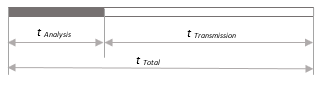Figure 1: Optimizing sensing and transmission times.

The aim of this work is to determine the optimal modulation classification algorithm and suggest the subset of the strongest and robust features derived from the received signal that could be used to blindly classify the modulation type in our hardware application: a software-defined radio-based network consisting of multiple digital cognitive radio nodes. SDR-based nodes are operating in the frequency band from 70 MHz to 6 GHz with up to 56 MHz of instantaneous bandwidth are used as the hardware platform for the cognitive functionality deployment with FHSS capabilities. Available computational resources are Dual-core ARM Cortex A9 CPU, 2×512 MB of DDR3L RAM, and 512 MB of QSPI flash memory. The operation system is Embedded Linux. The radio part is based on Analog Devices AD9364 radio transceiver and Xilinx’ Zynq-7020 FPGA. It is supporting multiple digital modulations including both linear: QPSK, BPSK, 8PSK, 16PSK, and non-linear: 2FSK. Symbol rate could be also adjusted between 10 KSymbols/s and 1 MSymbol/s to generate the cognitive waveform. Our target application predefines most of the boundary conditions and operational requirements such as required decision-making speed and computational resources available. In this work time required for radio scene analysis t_Analysis is defined as a sum of time required for radio scene observation t_Observation and processing t_Processing for the received signal on the receiver front end. Time allocated for the active data transmission is data transmission time, t_Transmission and total time is the sum of observation and transmission time as illustrated by Figure 8. Allocating the sensing time and transmission time at the MAC layer is involving a tradeoff between ensuring the PUs user’s QoS requirements as opposed to maximizing the data throughput. To meet real-time operation requirements on the target hardware the following real-time performance characteristics must be met by the proposed algorithms. The maximum time available for radio-scene environment observation is t_observation=500×10^-6 seconds. Our application is a time-slotted communication system, where 500 microseconds corresponds to one-time slot, also maximum processing time has been selected likewise t_processing=500×10^-6 seconds, which requires the minimum classification speed of 2000 objects per second. Modulation classification is required to be performed for SNR values above the demodulation threshold of 12 dB, which corresponds to bit-error-rate BER=10^-8 and BER=3.4×10^-5 for BPSK and 2FSK, respectively.

The frequency of the radio scene environment sensing (how often sensing should be performed by the cognitive radio) and sensing time (the duration the sensing is performed) are key parameters affecting the throughput. While higher sensing times ensure more accurate radio scene environment sensing, this may result in a comparatively smaller duration for actual data transmission during the total time for which the spectrum may be used, thereby lowering the throughput [13]. To achieve the optimum between sensing time and throughput, for example, in IEEE 802.22 two-stage sensing (TSS) mechanism is implemented that includes: fast sensing, done at the rate of 1 ms/channel, and fine sensing performed on-demand. In this work, we have evaluated the possibility to perform the classification based on instantaneous values to shorten the spectrum sensing time and reduce computational costs. To improve classification accuracy, classification based on spectral-based statistical features derived from the wavelet transform of the received signal observed during the certain observation time frame has been proposed. In this study observation times of 100 and 500 microseconds have been used. The lowest observation time has been selected 100 microseconds to accommodate the lowest symbol rate of 10 KSymbols/second supported in our target application for cognitive waveform generation.

Figure 2:  Modulation classification using a) instantaneous values of the time domain signal input; b) time series statistics input.

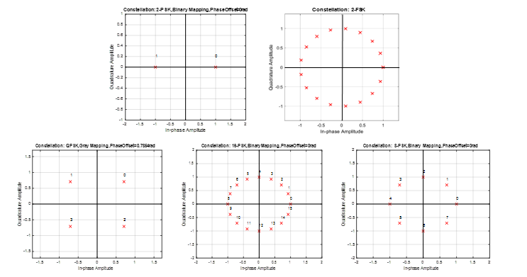Figure 3: Constellation plots for studies modulation classes BPSK, 2FSK, QPSK, 8PSK, 16PSK.

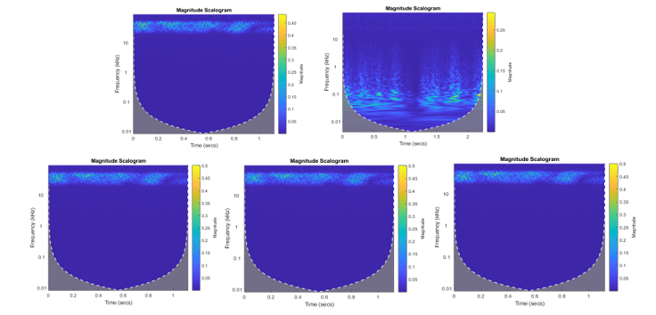Figure 4: Scalograms obtained from Haar transform. wavelet coefficients for BPSK, 2FSK, QPSK, 8PSK, 16PSK. Observation time 500 microseconds signal.

The highest: 500 microseconds that correspond to one time slot in our time-slotted target application. Wavelet transform has been used in this work for the feature extraction, since obtained wavelet coefficients could be reused also to detect the vacant frequency channels and estimate the symbol rate, what could potentially save time and computational resources spent on radio scene analysis.  Cyclostationary based algorithms have also been named in the literature as a powerful algorithm for modulation type and symbol rate estimation and vacant frequency channels detection. However, they are prone to cyclostationary noise and require longer observation time and is relatively computationally complex [14], and therefore this work has been focused on wavelet-based algorithms. Multiple supervised machine learning classifiers have been tested to perform classification based on instantaneous values and time-series statistics. The performance of tested classifiers has been evaluated in terms of classification accuracy and speed.

2. Methodology

Both feature extraction and classification algorithms applied in the literature to solve the modulation classification problem has been studied and evaluated. Primary, modulation type classification has been performed based on the input values of the instantaneous values of the in-phase and quadrature components of the time domain digital signal. Classification results have been satisfactory for the case of the binary classification between 2FSK and BPSK modulations. However, once the classification task has been extended to the higher-order modulations, the suggested classification approach has shown unacceptably low classification accuracy of 78.1 %. The highest classification accuracy of 84.9 % has been observed in the validation phase for classifying five modulations into two classes: linear and non-linear modulations using a fine SVM classifier.

Therefore, to improve the classification accuracy for higher-order modulations we have looked at multiple statistical features extracted from the time series containing the received signal observed during observation times of 100 and 500 microseconds. The following criteria have been considered when selecting classification features and feature extraction algorithm:

1. Robustness to noise; 2. Computational complexity; 3. Possibility to reuse preprocessed data for solving other radio scene environments observation tasks such as vacant bands detection and symbol rate estimation. Nine spectral-based statistical features derived from Haar wavelet transform coefficients calculated from the frequency domain signal observed during the selected observation time. The Haar transform has been selected as the simplest and less computationally demanding of all wavelet families. From the vector of wavelet coefficients, nine statistical features have been derived. To determine the strongest features to be used as inputs to ML classifier fractional factorial design analysis has been performed.

In statistics, a full factorial experiment is an experiment whose design consists of two or more factors, each with discrete possible values or “levels”, and whose experimental units take on all possible combinations of these levels across all studied factors.  Fractional factorial designs are experimental designs consisting of a carefully chosen subset or fraction of the experimental runs of a full factorial design. Significance is quantitively measured and referred to as the main effect [15]. A fractional factorial design approach has been used to analyze the main effects of every of nine statistical features and observation time on two studied response parameters: classification speed and accuracy in conditions of noise represented by two levels: AWGN and AWGN and multipath Rician channel model. Two levels have been applied and studied: first-level “-1” corresponds to not including the classification feature into classification and second level “+1” corresponds to including the studied feature into classification input. Observation time has also been varied according to two levels: first “-1“corresponds to 100 microseconds and the second level “+1” corresponds to 500 microseconds observation time. MATLAB and Simulink environment has been used for training and validation data sets generation including the modulator and propagation channel models, MathWorks classification learner ML Classification Learner tool has been used to train and validate classifiers. Twenty-four supervised ML classification algorithms have been studied and evaluated in terms of classification accuracy and classification speed for two studied channel models: AWGN and Rician multipath channels with AWGN.

3. Input data and feature extraction

To suggest optimal feature extraction and classification algorithms for our target radio application seven artificial data sets, consisting of signal samples modulated into 2FSK, BPSK, QPSK, 8PSK, 16PSK have been generated. Data sets are described in detail in Section 4. Figure 3 presents the constellation plots of five studied modulation types.

3.1. Classification using instantaneous values

The classification performed using instantaneous values of the time domain signal and SNR as classification inputs does not require any feature extraction: the raw values of the in-phase and quadrature component and SNR (recorded by transceiver as RSSI)  have been used directly as an input to the classifier.

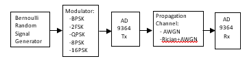Figure 5: Generalized model used for data set generation.

Table 1: Spectral-based features derived from time series used for modulation type classification

N	Feature	Factor	Description
1	Mean	A	Mean value of the wavelet coefficients obtained from single-level discrete wavelet transform of the frequency domain signal.
2	Standard Deviation	B	Standard deviation of the wavelet coefficients obtained from single-level discrete wavelet transform of the frequency domain signal.
3	Kurtosis	C	Kurtosis is a statistical measure that defines how heavily the tails of a distribution differ from the tails of a normal distribution calculated from the wavelet coefficients obtained from single-level discrete wavelet transform of the frequency domain signal [16].
4	Skewness	D	Skewness is a measure of the asymmetry of the probability distribution of a real-valued random variable about its mean. Calculated from the wavelet coefficients obtained from single-level discrete wavelet transform of the frequency domain signal [16].
5	Median absolute deviation	E	It is a measure of the statistical dispersion:  a robust measure of the variability of a univariate sample of quantitative data. It is more resilient to outliers in a data set than the standard deviation.  It is calculated from the wavelet coefficients obtained from single-level discrete wavelet transform of the frequency domain signal [17].
6	Root-mean-square level	F	The RMS value of a set of values (or a continuous-time waveform) is the square root of the arithmetic mean of the squares of the values, or the square of the function that defines the continuous waveform [18].
7	Zero crossing rate	G	It is the rate of sign-changes along a signal: the rate at which the signal changes from positive to zero to negative or from negative to zero to positive [19].
8	Interquartile range	H	The interquartile range (IQR) is a measure of variability: calculated based on dividing a data set into quartiles [20].
9	75th Percentile	I	The percentile rank of a score is the percentage of scores in its frequency distribution that are equal to or lower than it [21].
10	SNR	J	Signal-to-Noise ratio corresponds to RSSI value for the received signal measured by transceiver.

Table 2: Classifiers performance reached in validation. Classification between FSK and BPSK modulations. AWGN channel (SNR ranging from 1 to30 dB). Data set 1

Classifier	With PCA (1 feature of 3)		No PCA (3 features of 3)		No PCA (2 features of 3, No SNR)
	Average Accuracy, %	Prediction speed, Objects/s	Average Accuracy, %	Prediction speed, Objects/s	Average Accuracy, %	Prediction speed, Objects/s
Decision Trees: Fine	52.1	1600 000	86.0	1 200 000	84.2	2 000 000
Decision Trees: Medium	51.3	1200 000	85.2	1 000 000	83.3	2 100 000
Decision Trees: Coarse	50.7	1300 000	82.2	2 300 000	82.1	2 100 000
KNN: Fine	55.5	770 000	82.3	310 000	78.9	300 000
KNN: Medium	57.9	220 000	86.1	110 000	84.6	110 000
KNN: Coarse	61.5	55 000	86.8	28 000	85.5	27 000
KNN: Cosine	50.0	300	83.7	290	78.1	320
KNN: Cubic	57.9	150 000	86.1	29 000	84.6	46 000
KNN: Weighted	56.0	220 000	84.2	130 000	82.0	120 000
SVM: linear	50.1	47 000	55.3	3000	63.8	120 000
SVM: Quadratic	50.0	70 000	54.7	2300	42.8	92 000
SVM: Cubic	50.0	160 000	58.8	34 000	62.8	40 000
SVM: Fine  Gaussian	49.5	230	86.9	790	85.4	970
SVM: Medium  Gaussian	49.8	190	86.5	610	84.3	750
SVM: Coarse  Gaussian	49.8	240	49.8	240	81.4	600
Ensemble Boosted Trees	51.3	110 000	86.3	120 000	85.0	120 000
Ensemble Bagged Trees	55.5	19 000	85.4	44 000	83.1	33 000
Ensemble Subspace Discriminant	49.8	100 000	50.3	86 000	50.5	120 000
Ensemble Subspace KNN	55.5	34 000	80.5	6100	69.5	17 000
Ensemble RUS Boosted Trees	51.3	120 000	85.1	150 000	83.3	130 000
Logistic Regression	49.8	1600 000	50.9	1 200 000	50.5	3 200 000
Linear Discriminant	49.8	1200 000	50.3	1 900 000	50.5	1 300000

3.2. Classification using time-series statistics.

Nine spectral-based statistical features have been derived from the received signal observed during the observation time.  Primary fast Fourier transform has been applied to switch to the frequency domain. Then discrete wavelet transform has been applied to the frequency domain signal using Haar wavelet. This transform cross-multiplies a function against the Haar wavelet with various shifts and stretches. Figure 4 presents scalograms plots for studied modulations obtained by Haar wavelet transform. Then from the derived wavelet coefficients, nine spectral-based statistical features summarized in Table 1 have been calculated.

4. Data set

Seven data sets used for training and validation have been generated and are described briefly below. Three labeled artificial data sets consisting of three features:  instantaneous values of in-phase and quadrature components of the time domain signal and SNR and four data sets consisting of nine statistical features extracted from time-series recorded during 100 and 500 microseconds and SNR for two channel models: AWGN and Rician channel with AWGN. Figure 5 describes the generalized model used to generate data sets.

Data Set 1: Binary classification between BPSK and 2FSK using instantaneous values. Data set for training and validation has been generated using a virtual model presented in Figure 5.  The random input signal has been generated by Bernoulli binary random signal generator and modulated into BPSK or FSK. The modulated signal is transmitted by transmitter AD9364 TX. AWGN channel model has been selected to emulate the propagation environment, where SNR ranges from 30 to 1 dB.  Data set consisting of 408000 rows and 4 columns, where two first columns correspond to the instantaneous values of the signal in the time domain: in-phase and quadrature components, the third column corresponds to SNR value and the fourth column represents the data label. 80 % of the data set has been used for training the classifiers and 20 % has been used for validation.

Data Set 2:  Classification of BPSK, 2FSK, QPSK, 8PSK, 16PSK into two classes linear and nonlinear using instantaneous values. Data set of total size 910000 rows by 4 columns consisting of BPSK, 2FSK, QPSK, 8PSK, 16PSK has been generated in a similar way as Data Set 1: two first columns are corresponding to the instantaneous values of the signal in the time domain: in-phase and quadrature components, the third column corresponding to SNR value and the fourth column represents the data label corresponding to two classes: linear or non-linear modulation. Also, 80 % of the generated data set has been used for training the classifiers and 20 % of the generated data set has been used for validation of the classifiers.

Data Set 3:  Classification of BPSK, 2FSK, QPSK, 8PSK, 16PSK into five classes using instantaneous values. Data set 3 consisting of five modulations described above has been used to train classifiers to classify all five modulation types. In this data set only the fourth column corresponding to the label has been changed to accommodate five output classes. Also, 80 % of the data set has been used for training of the classifiers and 20% for validation.

Table 3: Classifiers performance reached in validation. Classification between linear and non-linear modulations.  Non-Linear: FSK, linear:  BPSK, QPS, 8PSK, 16PSK modulations. AWGN channel (SNR ranging from 1 to 30dB). Data set 2.

Classifier	Average Accuracy, (%)	Prediction speed, (Objects/s)
Decision Trees: Fine	80.5	1 200 000
Optimized Trees	83.0	3 400 000
KNN: Fine	77.1	310 000
KNN: Medium	82.6	110 000
SVM: Fine Gaussian	84.9	790
Ensemble Boosted Trees	80.9	120 000
Ensemble Bagged Trees	81.8	44 000
Ensemble Subspace KNN	80.5	6100
Ensemble RUS Boosted Trees	78.1	150 000

 Data Set 4: Classification of BPSK, 2FSK, QPSK, 8PSK, 16PSK into five classes using statistical features derived from time series observed during 500 microseconds for AWGN channel.

Data set 4 consists of 1500 samples (300 signal samples for every modulation type) resulting in a matrix of 1500 rows by 11 columns where the first nine columns correspond to statistical features column 10 corresponds to SNR and the last column corresponds to data class label.   Statistical features for every signal sample have been derived from the received signal observed during 500 microseconds in conditions of the AWGN propagation channel (SNR ranging from 1 dB to 30 dB). Also, 80 % of the data set has been used for training, and 20 % for validation.

Data Set 5: Classification of BPSK, 2FSK, QPSK, 8PSK, 16PSK into five classes using statistical features derived from time series observed during 100 microseconds. AWGN channel. Data set 5 consisting of 1500 samples (300 signal samples for every modulation type) resulting in a matrix of 1500 rows by 11 columns where the first nine columns correspond to statistical features, column 10 corresponds to SNR and the last column corresponds to data class label.  Statistical features for every signal sample have been derived from the received signal observed during 100 microseconds in conditions of AWGN propagation channel with

SNR ranging from 1 to 30 dB. Also, 80% of the data set has been used for training, and 20% for validation.

Data Set 6: Classification of BPSK, 2FSK, QPSK, 8PSK, 16PSK into five classes using statistical features derived from the received signal observed during 500 microseconds for Rician multipath channel. Data set 6 consisting of 1500 samples (300 signal samples for every modulation type) resulting in a matrix 1500 rows by 11 columns where the first nine columns correspond to statistical features, column 10 corresponds to SNR and the last column corresponds to data class label.  Statistical features have been derived from time-domain signal observed during 500 microseconds in conditions of Rician multipath line-of-sight fading channel model with AWGN (SNR = 30). Three fading paths have been chosen with path delays selected for outdoor environments 0; 9×10^-5 and 1.7×10^-5. Path delay ranging 10^-5 is suggested for the mountains area. Average path gains have been chosen [0 -2 -10]. The Rician K-factor has been selected K-factor = 4, it specifies the ratio of specular-to-diffuse power for a direct line-of-sight path, it is usually in the range [1, 10] and 0 corresponds to Rayleigh fading. Maximum Doppler shift has been chosen 4 dB, which corresponds to a signal from a moving pedestrian [22]. Also, 80% of the data set has been used for training the classifiers and 20 % for validation.

Data Set 7: Classification of BPSK, 2FSK, QPSK, 8PSK, 16PSK into five classes using statistical features derived from time series observed during 100 microseconds. Rician multipath channel. Data set 7 consisting of 1500 samples (300 signal samples for every modulation type) resulting in a matrix 1500 rows by 11 columns where the first nine columns correspond to statistical features column 10 corresponds to SNR and the last column corresponds to data class label.  Statistical features for every signal sample have been derived according to the steps summarized in feature extraction from time-domain signal observed during 100 microseconds in conditions of Rician multipath channel model with AWGN with SNR = 30 dB. The properties of the Rician channel have been selected the same as in data set 6. 80% of the data set has been used to train classifiers, 20% for validation.

Table 4: Classifiers performance reached in validation. Classification between FSK, BPSK, QPSK, 8PSK and 16PSK modulations using statistical features derived from the wavelet transform of the time series recorded during 500 microseconds. AWGN (SNR ranging from 1 to 30 dB) channel. Data set 4.

Classifier	With PCA (1 feature of 10)		No PCA (10 features of 10)		No PCA (5 features of 10)		No PCA Mean (1 features of 10)
	Average Accuracy, %	Prediction speed, Objects/s	Average Accuracy, %	Prediction speed, Objects/s	Average Accuracy, %	Prediction speed, Objects/s	Average Accuracy, %	Prediction speed, Objects/s
Decision Trees: Fine	100	15000	100	21000	100	20000	100	12000
Decision Trees: Medium	89.3	13000	99.7	23000	90.6	21000	79.9	18000
Decision Trees: Coarse	82.9	15000	88.1	19000	68.9	23000	67.5	19000
KNN: Fine	100	22000	100	42000	100	48000	100	51000
KNN: Medium	98.1	22000	96.6	26000	98.2	38000	97.2	56000
KNN: Coarse	80.6	18000	61.1	13000	61.7	21000	69.1	36000
KNN: Cosine	38.3	18000	96.9	22000	97.2	33000	21.3	38000
KNN: Cubic	98.1	17000	96.6	7800	98.5	20000	97.2	52000
KNN: Weighted	100	18000	100	36000	100	52000	100	52000
SVM: linear	57.0	15000	93.8	18000	75.1	21000	63.8	28000
SVM: Quadratic	51.2	20000	100	17000	98.0	17000	51.8	22000
SVM: Cubic	59.5	16000	100	16000	100	17000	47.7	27000
SVM: Fine Gaussian	79.9	13000	100	12000	99.2	16000	75.9	18000
SVM: Medium Gaussian	81.4	9400	97.9	16000	85.0	18000	69.4	20000
SVM: Coarse Gaussian	52.1	8200	88.9	14000	67.8	14000	65.9	16000
Ensemble Boosted Trees	93.0	9200	52.8	27000	99.9	10000	82.1	11000
Ensemble Bagged Trees	100	8200	100	11000	100	11000	100	12000
Ensemble Subspace Discriminant	56.3	6100	69.9	5900	59.3	6200	70.6	9500
Ensemble Subspace KNN	100	4400	100	4500	100	5000	100	6700
Ensemble RUS Boosted Trees	90.5	9800	83.6	61000	95.3	13000	80.4	11000
Linear Discriminant	56.3	13000	77.4	17000	62.5	17000	70.6	17000
Naïve Bayes	48.8	28000	60.9	60000	86.0	4800	73.8	18000

Table 5: Classifiers performance reached in validation. Classification between FSK, BPSK, QPSK, 8PSK and 16PSK modulations using statistical features derived from the wavelet transform of the time series recorded during 500 microseconds for Richian multipath with AWGN (SNR =30dB) channel model. Data set 5.

Classifier	With PCA (1 feature of 10)		No PCA (10 features of 10)		No PCA (5 features of 10)		No PCA Mean (1 feature of 10)
	Average Accuracy, %	Prediction speed, Objects/s	Average Accuracy, %	Prediction speed, Objects/s	Average Accuracy, %	Prediction speed, Objects/s	Average Accuracy, %	Prediction speed, Objects/s
Decision Trees: Fine	100	21000	100	27000	100	150000	93.0	160000
Decision Trees: Medium	49.5	98000	60.9	140000	55.6	150000	40.8	140000
Decision Trees: Coarse	41.6	11000	45.2	110000	41.5	120000	31.1	150000
KNN: Fine	100	22000	100	40000	100	79000	100	72000
KNN: Medium	95.7	23000	96	25000	95.7	45000	95.4	71000
KNN: Coarse	34.5	18000	36	16000	42.5	30000	37.7	36000
KNN: Cosine	37.7	17000	95.7	36000	95.7	30000	21.3	34000
KNN: Cubic	95.7	24000	95.6	2400	95.3	17000	95.4	54000
KNN: Weighted	100	29000	100	35000	100	38000	100	81000
SVM: linear	36.1	21000	36.6	26000	36.1	26000	21.8	40000
SVM: Quadratic	35.7	17000	66.6	21000	45.2	26000	23.5	29000
SVM: Cubic	36.5	19000	100	21000	61.4	30000	23.2	33000
SVM: Fine Gaussian	37.1	7800	91.8	11000	81.6	14000	38.0	11000
SVM: Medium Gaussian	36.2	8700	46.0	10000	44.2	11000	29.6	12000
SVM: Coarse Gaussian	35.0	8500	35.1	9700	34.9	11000	24.3	9700
Ensemble Boosted Trees	56.8	9400	86.4	12000	85.4	9700	49.9	12000
Ensemble Bagged Trees	100	9300	100	14000	100	8700	100	10000
Ensemble Subspace Discriminant	35.8	7800	39	8100	35.0	6400	22.5	8400
Ensemble Subspace KNN	100	5700	100	5300	100	4100	100	6100
Ensemble RUS Boosted Trees	61.7	11000	80.5	14000	86.0	14000	47.5	13000
Linear Discriminant	35.8	8600	37.9	18000	34.7	110000	22.5	100000
Naïve Bayes	39.9	9700	37.6	74000	37.9	110000	24.9	140000

5. ML classifiers training and validation results

Selected twenty-three classifiers have been trained and validated multiple times using every data set described above to investigate the effect of the extracted features and observation time on classification accuracy and speed. Among the trained classifiers we have studied decision trees, KNN with the various kernels, support vector machines (SVM), ensembles with bagging and boosting sampling, and discriminant methods. Also, principal component analysis PCA has been applied to keep enough components to explain 95 % of data variance for the dimension reduction. To protect against overfitting five-fold cross-validation method was used.

5.1. Classification using instantaneous values

Modulation type classification has been performed based on the input values of the instantaneous values of the in-phase and quadrature components of the time domain digital signal. Primary Classifiers have been trained three times using data set 1: 1. using PCA, 2. Using all three features: in-phase, quadrature components and SNR 3. Using two features including in-phase, quadrature components. Table 2 summarizes the validation results for the AWGN channel with SNR ranging from 1 to 30 dB. The effect of input features available in the data set 1 on classification accuracy, and speed has been studied. The highest classification accuracy has been achieved using all three available features: in-phase, quadrature components, and SNR. However, removing SNR from classification resulted in a reduction in the average classification accuracy by only 3 %. The highest average classification accuracy of 86.9 % was observed for the Fine Gaussian SVM, which on the other hand has been observed to be the slowest. Ensemble boosted trees with 30 decision trees learners trained using AdaBoost sampling and 20 splits and fine decision trees have shown optimal performance in terms of both classification accuracy and speed with an average classification accuracy of 86.3 % and 86.0 %, classification speed of 1200000 objects per second, which is faster than required 2000 objects per second.

Data set 3 containing also instantaneous values of the time domain signal and SNR consisting of five modulations has been used to train classifiers to classify all five modulation types. However, the average classification accuracy has not met the requirement of 85 %. The highest classification accuracy of 78.1 % has been reached by customized decision trees with the number of splits set to 2689, Gini’s diversity index has been used as a split criterion.

Among the other tested classifiers, there were ensemble bagged trees, ensemble boosted trees, RUS boosted trees which have demonstrated even worse classification accuracy than decision trees. To capture more of the fine differences between the received signal modulated into different linear modulations it is suggested to use the spectral features derived from the signal observed during the selected observation time.

5.2. Classification using time-series statistics.

Training and validation for both propagation channels AWGN (SNR from 1 dB to 30 dB) and AWGN (SNR = 30 dB) with Rician fading have been performed using data sets 4-7. Primary, the training of the studied classifiers has been performed using time series recorded during observation time corresponding to 500 microseconds using data sets 4 and 5 for AWGN and Rician channel with AWGN, respectively. Classifiers have been trained four times: 1. using PCA, 2. Using all ten spectral-based statistical features 3. Using five features including mean, standard deviation, root-mean-square level, zero crossing rate, 75^th percentile of a data set, and 4. Using only one input feature: the mean value of the wavelet coefficients. Tables 4-5 summarize the validation results for the AWGN channel with SNR ranging from 1 to 30 dB and Rician multipath with AWGN (SNR = 30 dB) channel. The best performing classifiers that have reached 100% classification accuracy have been retrained on the features derived from the time series observed during 100 microseconds. Tables 6 and 7 present the validation results for AWGN and multipath Rician channel trained and validated four times as for the time series recorded during 500 microseconds. Tables 6 and 7 show that four out of the five selected classifiers including fine decision trees, fine KNN, ensemble bagged trees, and ensemble subspace KNN that demonstrated classification accuracy of 100 % on the time series recorded during 500 microseconds have demonstrated classification accuracy close to 100 % when trained using PCA, using all ten features and using five features for both AWGN and  multipath channel also when have been trained on time series recorded during 100 microseconds. However, SVM has shown worse performance when trained with a reduced number of features.

Applying PCA has resulted in a drastic decrease in the classification accuracy for ensemble subspace KNN for both AWGN and multipath Rician channels. For most classifiers, like fine decision trees, ensemble bagged trees applying PCA has resulted in the decreased classification speed. Fine KNN has shown 100% classification accuracy for classification using only one input to the classifier: mean value and the highest classification speed of 56000 and 91000 objects/s for AWGN and multipath fading channel, respectively. However, KNN is still slow even using only one feature than fine decision trees using five features classifying 110000 and 120000 for AWGN and multipath channel.

6. Classification feature analysis using fractional factorial design

The fractional factorial design has been applied to determine the most significant classification features referred to as the design.

Table 6: Classifiers performance reached in validation. Classification between FSK, BPSK, QPSK, 8PSK and 16PSK modulations using statistical features derived from the wavelet transform of the time series recorded during 100 microseconds for AWGN (SNR ranging from 1 to 30 dB) channel. Data set 6

Classifier	With PCA (1 feature of 10)		No PCA (10 features of 10)		No PCA (5 features of 10)		No PCA Mean (1 feature of 10)
	Average Accuracy, %	Prediction speed, Objects/s	Average Accuracy, %	Prediction speed, Objects/s	Average Accuracy, %	Prediction speed, Objects/s	Average Accuracy, %	Prediction speed, Objects/s
Decision Trees: Fine	100	9500	100	18000	100	110000	100	120000
KNN: Fine	100	21000	100	37000	98.6	19000	100	56000
KNN: Weighted	100	22000	100	34000	100	47000	100	58000
SVM: Cubic	95.7	23000	100	19000	100	24000	38.7	31000
Ensemble Bagged Trees	100	7600	100	8700	100	6800	100	11000
Ensemble Subspace KNN	36.4	5500	100	4700	100	4800	100	5400

Table 7: Classifiers performance reached in validation. Classification between FSK, BPSK, QPSK, 8PSK and 16PSK modulations using statistical features derived from the wavelet transform of the time series recorded during 100 microseconds for Rician multipath with AWGN (SNR = 30dB) channel model. Data set 7

Classifier	With PCA (1 feature of 10)		No PCA (10 features of 10)		No PCA (5 features of 10)		No PCA Mean (1 feature of 10)
	Average Accuracy, %	Prediction speed, Objects/s	Average Accuracy, %	Prediction speed, Objects/s	Average Accuracy, %	Prediction speed, Objects/s	Average Accuracy, %	Prediction speed, Objects/s
Decision Trees: Fine	100	15000	100	23000	100	120000	94.2	160000
KNN: Fine	100	27000	100	24000	100	55000	100	91000
KNN: Weighted	100	25000	100	27000	100	48000	100	58000
SVM: Cubic	100	7900	100	16000	69.9	28000	69.9	28000
Ensemble Bagged Trees	100	5700	100	9900	100	11000	100	11000
Ensemble Subspace KNN	36.4	6900	100	5200	100	5000	100	6500

Table 8: Experimental factors and levels

N	Factor	Unit	Sym-bol	Coded level
				-1	+1
1	Mean	–	A	On	off
2	Standard Deviation	–	B	On	off
3	Kurtosis	–	C	On	off
4	Skewness	–	D	On	off
5	Median absolute deviation	–	E	On	off
6	Root-mean-square level	–	F	On	off
7	Zero crossing rate	–	G	On	off
8	Interquartile range	–	H	On	off
9	75th percentile of  data set	–	I	On	off
10	SNR	dB	J	On	off
11	Observation time	μs	K	100	500

factors that have the highest main effect on the response parameters: classification accuracy and speed We have been looking at both the main effects of the independent variables and interactions between the input parameters (A-J) and observation time (K) for the best performing classifier in terms of accuracy and speed. We have 10 design factors corresponding to the features referred as (A-J) and observation time referred to as (K) with 2 levels for each design factor corresponding to: high (+1) the feature is used for classification or low  (-1) the feature is not used for classification. Observation time has been also varied at two levels (+1) high corresponding to 500 microseconds and (-1) low corresponding to 100 microseconds. We have considered one noise factor corresponding to the propagation channel model with two levels corresponding to the AWGN (-1) channel with SNR ranging from 1dB to 30 dB and Rician multipath propagation and AWGN with SNR=30 dB (+1). The full factorial design will result in 2¹⁰ number of experiments, to reduce the number of experiments this study has been limited to fractional factorial design with 13 experiment runs performed, where the first ten runs with only one feature used for classification independently from the others for 100 microseconds observation time, since we are mostly interested to study the performance for the shortest observation time. The eleventh run has been selected to investigate the effect of observation time; the twelfth and thirteenth runs have been included to study the effect of observation time independently from the classification features with all nine spectral-based statistical features used as classification input.

The main effect is defined as the overall effect of an independent variable in the complex design. The definition of an effect is the difference in the means between the high (+1) and the low level (-1) of a factor. From this notation, A is the difference between the mean values of the observations at the high level of A minus the average of the observations at the low level of A. Interaction is defined here as the effect of one independent variable depending on the other independent variable, i.e it describes the combined effect of the independent variables considered simultaneously [15]. Tables 9-13 summarize the experimental design and results: main effect of every factor on classification accuracy and speed for five best performing classifiers: fine decision trees, fine KNN, weighted KNN, ensemble bagged trees with 59886 splits, and 30 learners and ensemble subspace KNN with 9 subspace dimensions and 30 learners.

The overall highest main effects on classification accuracy and speed have been observed for the fine decision trees classifier. In tables 9-13, we have obtained a relatively high main effect for using/not using SNR for classification. In tables 9-13, summarizing the performance of the classifier, it is possible to see that removing the SNR value as an input to the classifier does not affect the response parameters significantly, on the other hand using SNR value only for classification as in the experiment run N10  (what in reality does not make any sense) result in the very low classification accuracy. Since the main effect is a difference between the mean values of the high and low, we observe here the high main effect of SNR as a classification input parameter. For example, the main effect of using SNR (J) as classification input on classification accuracy for fine decision trees is –20.0, while for Kurtosis (C) it is 19.6. Classification accuracy if we use only (C) for classification experiment run N3 is 100% for both Rician and AWGN channels and if we use only (J) for classification is 8.6% for both Rician and AWGN channels. This makes the highest main effect of SNR input a questionable result for practical application. Also, the value of the main effect should be interpreted only in combination with the value of the response parameter: classification accuracy and speed.

The highest classification speed of 170 000 objects per second for 100% classification accuracy has been demonstrated by fine decision trees using only one classification input the skewness of the wavelet coefficients derived from signal observed during 100 microseconds for AWGN channel model. For Rician and AWGN, channel classification speed has been slower 130 000 objects/s. Both skewness and kurtosis has shown the highest main effect on classification accuracy for fine trees. Using mean value as the only input parameter to fine trees classifier, however, has shown less robust results in terms of the classification accuracy: 94.5% has been demonstrated for Rician and AWGN channel, while for AWGN channel 100%. The mean value shows the second-highest main effect on the classification accuracy 19.5 for the fine decision trees and the highest main effect of 10.9, 11.1, 11.5, and 10.9 for the other four classifiers including fine KNN, weighted KNN, ensemble bagged trees and ensemble subspace KNN, respectively. It also shows the highest main effect on the classification speed for all five selected classifiers.

Slightly slower classification speed has been demonstrated by KNN classifiers: 110000 objects per second have been observed for fine KNN for AWGN channel and 89000 objects per second for AWGN channel with Rician multipath. The slowest from all studied are ensembles, for example, ensemble subspace KNN has demonstrated a classification speed of 4500-6800 objects per

second. However, classification speed for ensembles does not decrease as much as for the fine trees with the increasing number of features. For ensemble bagged trees for AWGN channel the same classification speed of 11000 has been demonstrated for classification using only mean A and using all calculated features (A-J).

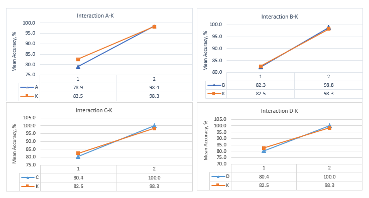
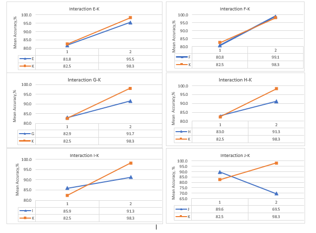Figure 6: Main Effects and interactions between factors (A-J) and observation time (K) for fine decision trees

Table 9: Experimental design and results of fractional factorial design limited to 13 experimental runs for fine decision trees classifier.

Factors. Fine Trees												AWGN		AWGN + Rician		Mean Accuracy	STD Accuracy	Mean Speed	STD Speed
Run	A	B	C	D	E	F	G	H	I	J	K	Speed	Accuracy	Speed	Accuracy
1	+	–	–	–	–	–	–	–	–	–	–	100000	100	160000	94.5	97.3	3.9	130000	113068
2	–	+	–	–	–	–	–	–	–	–	–	140000	100	140000	92.9	96.5	5.0	140000	98927
3	–	–	+	–	–	–	–	–	–	–	–	110000	100	150000	100	100.0	0.0	130000	105995
4	–	–	–	+	–	–	–	–	–	–	–	170000	100	130000	100	100.0	0.0	150000	91853
5	–	–	–	–	+	–	–	–	–	–	–	130000	93.8	98000	78.9	86.4	10.5	114000	69235
6	–	–	–	–	–	+	–	–	–	–	–	110000	100	140000	92.9	96.5	5.0	125000	98927
7	–	–	–	–	–	–	+	–	–	–	–	170000	75.4	130000	74.5	75.0	0.6	150000	91871
8	–	–	–	–	–	–	–	+	–	–	–	130000	72.9	160000	74.9	73.9	1.4	145000	113085
9	–	–	–	–	–	–	–	–	+	–	–	120000	73.4	99000	74.1	73.8	0.5	109500	69951
10	–	–	–	–	–	–	–	–	–	+	–	110000	8.6	180000	8.6	8.6	0.0	145000	127273
11	+	–	–	–	–	–	–	–	–	–	+	12000	100	160000	93	96.5	4.9	86000	113069
12	+	+	+	+	+	+	+	+	+	+	–	18000	100	23000	100	100.0	0.0	20500	16193
13	+	+	+	+	+	+	+	+	+	+	+	21000	100	27000	100	100.0	0.0	24000	19021
Main Effects Accuracy	19.5	16.5	19.6	19.6	13.7	18.3	8.7	8.3	5.4	-20.0	15.7
Main Effects Speed	-69.2	-29.6	-29.5	-27.5	-35.6	-31.1	-35.8	-36.7	-40.3	-58.4	-24.7

Table 10: Experimental design and results of fractional factorial design limited to 13 experimental runs for fine KNN classifier

Factors Fine KNN												AWGN		AWGN + Richian		Mean Accuracy	STD Accuracy	Mean Speed	STD Speed
Run	A	B	C	D	E	F	G	H	I	J	K	Speed	Accuracy	Speed	Accuracy
1	+	–	–	–	–	–	–	–	–	–	–	73000	100	91000	100	100.0	0.0	36500	64276
2	–	+	–	–	–	–	–	–	–	–	–	69000	100	41000	100	100.0	0.0	55000	28921
3	–	–	+	–	–	–	–	–	–	–	–	83000	100	65000	100	100.0	0.0	74000	45891
4	–	–	–	+	–	–	–	–	–	–	–	54000	100	77000	100	100.0	0.0	65500	54377
5	–	–	–	–	+	–	–	–	–	–	–	91000	100	84000	100	100.0	0.0	87500	59326
6	–	–	–	–	–	+	–	–	–	–	–	110000	100	86000	100	100.0	0.0	98000	60740
7	–	–	–	–	–	–	+	–	–	–	–	72000	79.9	69000	80.6	80.3	0.5	70500	48734
8	–	–	–	–	–	–	–	+	–	–	–	80000	100	110000	100	100.0	0.0	95000	77711
9	–	–	–	–	–	–	–	–	+	–	–	83000	100	110000	100	100.0	0.0	96500	77711
10	–	–	–	–	–	–	–	–	–	+	–	93000	21.3	83000	21.3	21.3	0.0	88000	58675
11	+	–	–	–	–	–	–	–	–	–	+	51000	100	72000	100	100.0	0.0	61500	50841
12	+	+	+	+	+	+	+	+	+	+	–	37000	100	30000	100	100.0	0.0	33500	21142
13	+	+	+	+	+	+	+	+	+	+	+	42000	100	40000	100	100.0	0.0	41000	28214
Main Effects Accuracy	10.9	9.8	9.8	9.8	9.0	9.8	1.3	9.8	9.8	-24.3	9.0
Main Effects Speed	-38.0	-34.1	-25.9	-29.6	-20.1	-15.5	-27.4	-16.8	-16.2	-19.8	0.0

Table 11: Experimental design and results of fractional factorial design limited to 13 experimental runs for weighted KNN classifier.

FactorsWeighted												AWGN		AWGN + Rician		Mean Accuracy	STD Accuracy	Mean Speed	STD Speed
Run	A	B	C	D	E	F	G	H	I	J	K	Speed	Accuracy	Speed	Accuracy
1	+	–	–	–	–	–	–	–	–	–	–	62000	100	58000	100	100.0	0.0	60000	40941
2	–	+	–	–	–	–	–	–	–	–	–	63000	100	67000	100	100.0	0.0	65000	47305
3	–	–	+	–	–	–	–	–	–	–	–	90000	100	63000	100	100.0	0.0	76500	44477
4	–	–	–	+	–	–	–	–	–	–	–	62000	100	77000	100	100.0	0.0	69500	54377
5	–	–	–	–	+	–	–	–	–	–	–	66000	100	55000	100	100.0	0.0	60500	38820
6	–	–	–	–	–	+	–	–	–	–	–	73000	100	79000	100	100.0	0.0	76000	55791
7	–	–	–	–	–	–	+	–	–	–	–	60000	79.4	67000	100	89.7	14.6	63500	47313
8	–	–	–	–	–	–	–	+	–	–	–	71000	100	79000	80	90.0	14.1	75000	55798
9	–	–	–	–	–	–	–	–	+	–	–	68000	100	72000	100	100.0	0.0	70000	50841
10	–	–	–	–	–	–	–	–	–	+	–	56000	20.4	73000	21.3	20.9	0.6	64500	51604
11	+	–	–	–	–	–	–	–	–	–	+	52000	100	81000	100	100.0	0.0	66500	57205
12	+	+	+	+	+	+	+	+	+	+	–	34000	100	23000	100	100.0	0.0	28500	16193
13	+	+	+	+	+	+	+	+	+	+	+	36000	100	35000	100	100.0	0.0	35500	24678
Main Effects Accuracy	11.1	9.9	9.9	9.9	9.9	9.9	5.5	5.6	9.9	-24.4	9.0
Main Effects Speed	-21.3	-25.2	-20.2	-23.3	-27.2	-20.4	-25.9	-20.9	-23.0	-25.4	-14.1

Table 12: Experimental design and results of fractional factorial design limited to 13 experimental runs for Ensemble bagged trees classifier.

FactorsEnsemble Bagged Trees												AWGN		AWGN + Rician		Mean Accuracy	STD Accuracy	Mean Speed	STD Speed
Run	A	B	C	D	E	F	G	H	I	J	K	Speed	Accuracy	Speed	Accuracy
1	+	–	–	–	–	–	–	–	–	–	–	11000	100	11000	100	100.0	0.0	11000	7707
2	–	+	–	–	–	–	–	–	–	–	–	9400	100	9600	100	100.0	0.0	9500	6718
3	–	–	+	–	–	–	–	–	–	–	–	11000	100	12000	100	100.0	0.0	11500	8415
4	–	–	–	+	–	–	–	–	–	–	–	10000	100	11000	100	100.0	0.0	10500	7707
5	–	–	–	–	+	–	–	–	–	–	–	10000	100	10000	100	100.0	0.0	10000	7000
6	–	–	–	–	–	+	–	–	–	–	–	11000	100	10000	100	100.0	0.0	10500	7000
7	–	–	–	–	–	–	+	–	–	–	–	12000	76	7700	100	88.0	17.0	9850	5382
8	–	–	–	–	–	–	–	+	–	–	–	9800	100	8500	100	100.0	0.0	9150	5940
9	–	–	–	–	–	–	–	–	+	–	–	7600	100	7700	100	100.0	0.0	7650	5374
10	–	–	–	–	–	–	–	–	–	+	–	14000	8.9	1200	8.7	8.8	0.1	7600	842
11	+	–	–	–	–	–	–	–	–	–	+	12000	100	10000	100	100.0	0.0	11000	7000
12	+	+	+	+	+	+	+	+	+	+	–	8700	100	9900	100	100.0	0.0	9300	6930
13	+	+	+	+	+	+	+	+	+	+	+	11000	100	14000	100	100.0	0.0	12500	9829
Main Effects Accuracy	11.5	10.3	10.3	10.3	10.3	10.3	5.1	10.3	10.3	-29.2	9.4
Main Effects Speed	1.4	0.6	1.4	1.0	0.8	1.0	0.7	0.4	-0.2	-0.3	2.1

Table 13: Experimental design and results of fractional factorial design limited to 13 experimental runs for Ensemble subspace KNN classifier

FactorsEnsemble Subspace KNN												AWGN		AWGN + Rician		Mean Accuracy	STD Accuracy	Mean Speed	STD Speed
Run	A	B	C	D	E	F	G	H	I	J	K	Speed	Accuracy	Speed	Accuracy
1	+	–	–	–	–	–	–	–	–	–	–	6100	100	6500	100	100.0	0.0	6300	4525
2	–	+	–	–	–	–	–	–	–	–	–	6200	100	6200	100	100.0	0.0	6200	4313
3	–	–	+	–	–	–	–	–	–	–	–	6800	100	7100	100	100.0	0.0	6950	4950
4	–	–	–	+	–	–	–	–	–	–	–	5600	100	6400	100	100.0	0.0	6000	4455
5	–	–	–	–	+	–	–	–	–	–	–	6700	100	6800	100	100.0	0.0	6750	4738
6	–	–	–	–	–	+	–	–	–	–	–	6600	100	6200	100	100.0	0.0	6400	4313
7	–	–	–	–	–	–	+	–	–	–	–	6500	79.9	7800	100	90.0	14.2	7150	5452
8	–	–	–	–	–	–	–	+	–	–	–	6100	100	5900	80.6	90.3	13.7	6000	4108
9	–	–	–	–	–	–	–	–	+	–	–	6800	100	5500	100	100.0	0.0	6150	3818
10	–	–	–	–	–	–	–	–	–	+	–	6200	21.3	5300	21.3	21.3	0.0	5750	3733
11	+	–	–	–	–	–	–	–	–	–	+	6700	100	6100	100	100.0	0.0	6400	4243
12	+	+	+	+	+	+	+	+	+	+	–	4700	100	5200	100	100.0	0.0	4950	3606
13	+	+	+	+	+	+	+	+	+	+	+	4500	100	5300	100	100.0	0.0	4900	3677
Main Effects Accuracy	10.9	9.8	9.8	9.8	9.8	9.8	5.5	5.6	9.8	-24.3	9.0
Main Effects Speed	-0.7	-1.0	-0.7	-1.1	-3.0	-0.9	-0.6	-1.1	-1.1	-1.2	-0.6

Since the decision trees are the fastest classifier reaching an accuracy of 100%, the study of the interactions has been limited only to fine decision trees. Interaction between observation time and every of the spectral-based statistical feature (A-J) has been studied and plotted in Figure 6. Non-parallel lines corresponding to the main effects in Figure 6 indicate the presence of interaction between spectrum observation time and all the studied features. The study of interactions between extracted features has been discarded because they have been extracted from the same source: Haar transforms coefficients derived from frequency domain signal and therefore are not considered to be fully independent variables. The most prominent interactions are observed between 75^th percentile and observation time, SNR as a classification feature and observation time, root-mean-square level and observation time, skewness and observation time, kurtoses, and observation time.

7. Conclusions and future work

In the scope of this work we have studied the possibility to classify the modulation type using instantaneous values of the time domain signal and SNR as inputs to the classifier. The main advantage of this approach is that it has potential to increase throughput by shortening the spectrum observation time and decreases the computational complexity: the raw values of in-phase and quadrature components of the signal are used as an input to the classifier and therefore there is no need for any preprocessing or feature extraction. This approach is applicable for binary classification between BPSK and 2FSK modulations, however it fails in case the classification task is extended to multiple classes containing higher order modulations. The possible reason for this is the missing data that is not included in the pair of in-phase and quadrature component. If the input values pair lies on the x axis the modulation could be classified as any of four types: BPSK, 2FSK, 8PSK or 16PSK. In case of the input pairs are located on the y axis it could be classified as any of three modulation classes: 2FSK, 8PSK, 16PSK. We have confirmed that to reach the classification accuracy of at least 85% or higher for classification between multiple high order modulations it is required to observe the received signal and perform feature extraction. In this study we have studied nine spectral/based statistical features derived from the wavelet coefficients obtained by applying the Haar wavelet transform to the frequency domain received signal.  The highest classification speed of 170 000 objects/second and 100 % classification accuracy has been demonstrated by fine decision trees using as the single input kurtosis (C) derived from the wavelet coefficients derived from signal observed during 100 microseconds for AWGN channel. For line-of-sight fading Rician channel with AWGN demonstrated classification speed is slower 130 000 objects/s. Skewness and kurtosis have shown the highest main effect on classification accuracy for fine decision trees. The mean value demonstrated the highest main effects on classification speed for fine decision trees, fine KNN, weighted KNN, ensemble bagged trees, ensemble subspace KNN.

In the scope of the future work it is planned to implement the proposed fine decision trees classification algorithm on our target application hardware. Also, it is intended to extend this work to the multiple propagation channel models including Rayleigh and Rician for doppler shifts corresponding to target application embedded in the ground and aerial unmanned platforms moving with speeds 100-200 km/hour.