1. Introduction

Memory (LSTM) to forecast PV power for one hour ahead with an interval of five minutes. WPD is applied to split the PV power output time-series and next the LSTM is implemented to forecast high and low-frequency subseries. The results of this study indicate that the WPD-LSTM method outperforms in various seasons and weather conditions than LSTM, Gated Recurrent Units (GRU), RNN, and Multilayer Perceptron (MLP). Authors in [9] have presented a deep LSTM based on historical power data to predict the PV system output power for one hour ahead. The aim in [10] to suggest a hybrid model using LSTM and attention mechanism for short-term PV power forecasting, and employed LSTM to extract features from the historical data and learn in sequence the information on long-term dependence, to apply the attention mechanism trained at the LSTM to target the extracted relevant features, which has greatly enhanced the original predictive power of LSTM. An LSTM approach for short-term forecasts based on a timescale that includes global horizontal irradiance (GHI) one hour ahead and one day ahead have been applied in [11]. Furthermore, authors in [12] have implemented univariate and multivariate GRU models employing historical solar radiation, external meteorological variables, and cloud cover data to predict solar radiation. In [13], authors have presented multivariate GRU to predict Direct Normal Irradiance (DNI) hourly. And the suggested method is evaluated compared to LSTM using historical irradiance data. In addition, a hybrid deep learning model have introduced in [14] that combines a GRU neural network with an attention mechanism for solar radiation prediction. All these research contributions cited above are valuable. However, they are not able to identify the important parameters that would have an impact on the accuracy of predictions. and make real-time predictions for efficient and optimized management. Given the fluctuating nature of output power generation as a function of meteorological conditions such as the temperature, the wind speed, the cloud cover, the atmospheric aerosol levels and the humidity level, which leads to high uncertainties on the output power of PV [15]. Besides, according to the forecast horizon, PV forecasts range from very short to long term. In general, researchers focus on short-term, hourly and daily forecasts as opposed to long-term. The first are of major significance for the management of PVs and the related security constraints (planning, control of PV storage and the rapprochement of the electricity market, providing the secure operation of generation and distribution services, and reinforcing the security of grid operation), while the long-term forecasts are useful particularly, for maintenance [16]. In this context, we study the efficiency of three DL models. We also focus in this study, on real-time prediction of solar energy in order to help planner, decision-makers, power plant operators and grid operators to making responsive decisions as early as possible, and to manage smart grid PV systems more reliably and efficiently [17]. Moreover, the use of real-time prediction allows to adjust to changes in production and to react to complex events (exceptionally high or low load production or consumption). In addition, it decreases the amount of operating reserves needed by the system, thus reducing system balancing costs [18]. However, the models we have selected give good results and seem to be suitable for long-term forecasting thanks to their power as a deep learning model and their ability to perform complex processing on huge data sets. Moreover, we outline that our work has been experimented with Moroccan’s case, particularly in the region of Errachidia. In this perspective, Moroccan decision-makers have launched a global plan to improve the percentage of renewable energy in the energy mix and substantially improve energy efficiency. In view of increasing the percentage of electricity generation capacity from renewable energy sources (42% by 2020 and 52% by 2030) [19]. Therefore, we believe that the case of Morocco remains an interesting case study that could lead to important findings since it is not only a promising future PV energy supplier, but also one of the leading countries in the global energy transition, particularly in Africa. The remainder of this paper is organized into four sections. Section 2 gives an overview of our comparative methodology. Subsequently, section 3 presents the approach applied to elaborate the forecast models. Section 4 presents and discusses the obtained results. Finally, section 5 summarizes the conclusions and perspectives of this study.

2. Methodology

Solar energy prediction is a key element in enhancing the competitiveness of solar power plants in the energy market, and decreasing reliance on fossil fuels in socio-economic development. Our work aims to accurately predict the solar energy. For this purpose, we explore architectures of the RNN, LSTM and GRU algorithm which is suitable to be used for forecasting such time-series data, and we experiment and evaluate them in Morocco’s case, especially Errachidia area. This section presents at first the basis architecture of this recurrent neural network before explaining the important steps that we follow to build our models and perform our comparative study.

2.1        Recurrent Neural Network architecture

Recurrent neural network (RNN) is a category of neural network used in sequential data prediction where the output is dependent on the input [20]. The RNN [21] is capable to capture the dynamic of time-series data by storing information from previous computations in the internal memory. RNN has been applied in a context where past values of the output make a significant contribution to the future. It is mainly used in forecasting applications because of its ability to process sequential data of different length.

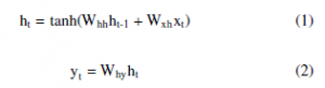
The basic principle of RNNs is to consider the input of a hidden neuron which takes input from neurons at the preceding time step [22]. To this purpose, they employ cells represented by gates that influence the output using historical data observations are given to generate the output. RNN is particularly efficient for learning the dynamic temporal behaviors exhibited in time-series data [23]. In RNN, the hidden neuron ht for a given input sequence x_t, it has information feedback from other neurons in the preceding time step multiplied by a W_hh which is the weight of the preceding hidden state h_t−1 can be calculated sequence by Eq.1. x_t is the input at instant time t, W_xh is the weight of the actual input state, tanh is the activation function. The output state y_t is computed according to the Eq.2 where W_hy is the weight at the output state.

The LSTM is a special kind of RNN, designed to avoid and resolve the vanishing gradient problems that limit the efficiency of simple RNN [8]. LSTM network has memory blocks that are connected through a succession of layers. In the LSTM cells, there are three types of gates: the input gate, the forget gate and the output gate. This makes it possible to achieve good results on a variety of time-series learning tasks, particularly in the nonlinear of a given dataset [24]. Each block of LSTM handles the state of the block and the output, it operates at different time steps and transmits its output to the following block and then the final LSTM block generates the sequential output [9]. Besides, LSTM is a robust algorithm, which allows the recurrent neural network to efficiently process time-series data. Its key component is memory blocks which have been released to address the vanishing gradient disadvantage by memorizing network parameters for long durations [25].an LSTM block gets an input sequence after that, the activation units are used by each gate to decide whether or not it is activated. This operation enables the change of state and the adding of information passing through the block conditional. In the training phase, the gates have weights that can be learned. In fact, the gates make the LSTM blocks smarter than conventional neurons and allow them to remember current sequences [10]. LSTM is flexible and estimates dependencies of different time scales thanks to its ability to perform long task sequences and to identify long-range features. Basically, LSTM starts with a forget gate layer (f_t) that uses a sigmoid function combined with the preceding hidden layer (h_t−1) and the current input (x_t) as described in the following equations:

where i_t, cˇ_t, f_t, o_t, c_t and h_t represent the input gate, cell input activation, forget gate, output gate, cell state, and the hidden state respectively. W_i, W_c, W_f and W_o represent their weight matrices respectively. b_i, b_c, b_f, and b_o represent the biases. x_t is the input, h_t-1 is the last hidden state, h_t is the internal state. σ is the sigmoid function.

2.2        Gated Recurrent Units architecture

The GRU [26] is a particular type of recurrent neural network proposed by Cho in 2014 which, is the same as the LSTM) in terms of use to resolve the issue of long-term memory network and backpropagation. The GRU network involves the design of several cells that store important information and forget those that are deemed irrelevant in the future [27]. The feedback loops of the GRU network can be regarded as a time loop, because the output of the cell from the past period is taken as an input in the following cell in addition to the actual input. This key property allows the model to remember the patterns of interest and to predict sequential time-series datasets over time. Unlike the LSTM, the GRU [28] consists of only two gates: update and reset gates. the GRU substitutes the forget gate and the input gate in the LSTM with an update gate that verifies the cell state of the previous state information that will be moved to the current cell, while, the reset gate defines whether new information will be included in the preceding state. For this reason, GRU has proven to be one of the most efficient RNN techniques, because of its capacity to learn and acquire dependencies over the long term and observations of varying length [29]. This characteristic is particularly useful for time-series data, and it is helpful in reducing the computational complexity [30]. GRU cells are described using the following equations:

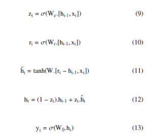
where z_t and r_t respectively correspond to the output of the up-

date gate and the reset gate, while W_z, W_r, W, and Wo respectively are the weights of each gate. σ and tanh respectively are the sigmoid and the hyperbolic tangent activation function, and x_t is the network input at time t. ht and h_t-1 correspond to the hidden layer information of the actual and precedent time, and hˆ_t is the candidate state of the input. Initially, the network input x_t at the time of the hidden state h_t-1 and t at the last state computes the output of the reset gate and the update gate by Eq.9 and 10. Next, after the reset of the reset gate r_t calculates the amount of memory stored, the implicit layer hˆ_t is computed by Eq.11, which is the new information at the actual time t. Then, by using Eq.12, the update gate z_z determines the amount of information was removed at the previous time, and how much information is stored in the candidate hidden layer ht at this time. The hidden layer information h_t is subsequently added. Finally, the output of the GRU is switched to the next GRU gated loop unit according to Eq.13: which is a sigmoid function.

3. Our approach for predicting solar energy

In this study, we apply three different DL models to predict the PV solar energy output, especially RNN, LSTM and GRU for the half-hour ahead. The aim of this study is to compares the relevance of the mentioned models, in order to identify the best algorithm to be used for predicting solar energy. The process of the method employed in this work is illustrated in Figure 1. It is organized into four main stages: data collection, data pre-processing, model training and parameterization, and model testing and validation. This section details how each of these processing/selection steps was performed, as well as key details on the architecture and parameters of the developed models.

Figure 1: Our method for predicting solar energy

3.1        Dataset

The datasets used in this work, they represent meteorological data of Errachidia province, which is situated in the sunny region of Morocco, it benefits from an important solar energy potential during all the year. This data consists of measurements from three years (2016, 2017 and 2018), and they are used to predict the solar energy level based on a set of measurable weather conditions, in purpose of analyzing the performance of the studied models.

3.2        Preprocessing and Feature Selection

Pre-processing and feature selection are fundamental steps in DL approaches for making collected data in an appropriate form. Preprocessing allows numerous tasks and operations to convert the source data in a clean data, in a way that it can be easily integrated into DL models. It impacts the accuracy of the model and its results. Feature selection provides the most appropriate features that properly affect the learning process, and can minimize the number of variables to efficiently enhance the accuracy of the model and avoid costly computations. Therefore, in this work, we proceed with the following steps to prepare and select features from the source data: extraction of target data inputs, selection of relevant features, filling in the null values, normalization of the data, and adjustment of the steps to be taken into account for prediction.

The source data give multiple features but not all of them are important for use in the prediction. In our case, we have selected four important features: solar energy, temperature, humidity and pressure. These features are the most and highly correlated variables to the targeted output (solar energy) according to Pearson correlations [31]. The objective of this step is to help developing most accurate models that learn from the most correlated data in order to give the most accurate forecasts. We note that we have selected the Median in order to fill missing data.

The features of a given dataset are usually presented at different scales. To ensure that all these values are at the same scale and to add uniformity to our dataset, we employ the Min-Max scale that transforms all values between 0 and 1, which removes the noise from our data and simplifying the learning process of our models.

Besides, the meteorological data are time-series with a time step of 30 min, and therefore, the actual data values are needed as inputs for making predictions. Time-series data cannot use future values as input features, whereas the inputs of a time-series model are the values of past features. In this work, we adjust our model to learn from the past to predict PV solar energy for the next half hour. This choice has been adopted because of the size of the data and to perform real-time predictions for an efficient and optimized management. Finally, based on best practices in the area of data analytics, the dataset is split into 80% and 20% were respectively used to train and test the models developed.

3.3        Training and models parametrization

Each of the models developed must be parameterized during the training phase in order to be able to provide the most accurate forecasts while taking into account the size of the batches. After setting different parameters for our DL models during the training and evaluating the results obtained, the Adam optimizer has proved to be the best optimizer and was then selected as the common parameter for all proposed DL models. ADAM, which is widely used and works better than other stochastic optimizers in empirical results [32], would allow the models to learn quickly. In addition, the tanh activation function has shown a good fitting for all DL models. On the other hand, we notice that our DL models have different architectures and that the number of layers and neurons for example has been fixed after tuning several values and selecting the ones that have given the best precisions. Figure 2 illustrates the neural network architecture, and Table 1 shows details on the architectures and the key parameters of each model suggested for the dataset studied.

Figure 2: ANN architecture for predicting solar energy Table 1: Architecture and parametrization of the models.

Models		Parameters
	Layers	Epocs	Activation Function	Optimizer	Batch size
RNN	RNN cell Of 100 units	20	Tanh	Adam	12719
LSTM	LSTM cell Of 100 units	20	Tanh	Adam	12719
GRU	GRU cell Of 100 units	20	Tanh	Adam	12719

3.4        Performance metrics

To evaluate the performance of the proposed DL models for PV solar energy prediction. A set of evaluation metrics widely-used are employed to evaluate the results accuracy forecasting. In this step, we have applied the most suitable to the context of DL and regression problems. For this purpose, five performance metrics, whose equations are presented below, have been employed for models testing as well as training: MAE (Mean Absolute Error), MSE (Mean Square Error), RMSE (Root Mean Square Error), Max Error (ME) and R squared (R²).

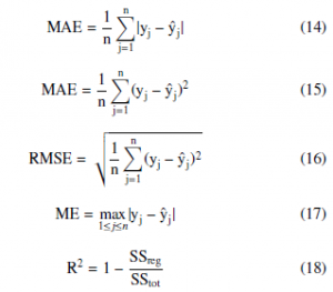
where y is the actual output, yˆ is the predicted output and n is the number of samples. Eq. 14 computes MAE as the average of the absolute errors (absolute values indicating the differences between the actual and the predicted values). Eq. 15 shows the MSE, which is the average squared errors (difference between the real values and what is estimated. Eq. 16 calculates RMSE, which is the square root of the MSE, and is applied in cases with small errors [33], whereas Eq. 17 measures the maximum residual error ME and reveals the worst error between the actual and predicted value. In addition, to calculate the predictive accuracy of proposed models, we also used R-squared, which is a statistical metric in a regression model, to identify the proportion of variance of the dependent variable that can be made explicit by the independent variable. Expressly, Eq. 18 indicates the R-squared measure to which the data correspond in the regression model (the goodness of fit) where SS_reg is the sum of the squares due to the regression and SS_tot is the total sum of the squares [34]. Eventually, in the different steps outlined in this section, we employed a set of technical tools for the implementation of the studied algorithms based on the Python libraries, including Pandas, NumPy, SciPy and Matplotlib in a Jupiter Notebook, in addition to Scikit-learn (sklearn) and TensorFlow.

4. Results and discussion

In this section, we present and discuss the results of our three studied models tested for PV solar energy forecasting. It should be noted that although R-squared (R²) is a commonly used metric, it is not regarded as an effective indicator of the models fit with the data [35]. A low or high R² value does not always indicate that the model is wrong or that it is automatically right [36]. Due to the controversy concerning the efficiency of R² as an appropriate metric for determining the best regression model [35, 36], we additionally evaluate our results using other statistical metrics that are the most widely used: MAE, MSE, Max Error and RMSE. The RMSE remains the most frequently employed in the regression area [37]. Table 2 show the metrics values corresponding to solar energy prediction in real time of studied models. Considering the parameters presented in Table 2, we can see the results for one-half hour ahead prediction of our experiments for the recurrent neural networks: RNN, LSTM and GRU. In spite of their architectural differences, RNN and LSTM have demonstrated similar performance, showing that the better model is strongly dependent on the task. Thanks to their ability to handle long-term dependencies in sequential information for timeseries predicting applications, both RNN and LSTM perform better with very high accuracy as shown by their related R² values which are respectively equal to 94.68% and 94.26%. GRU gives slightly less performance than the RNN and LSTM with 90.32 as value. It also causes errors unlike RNN and LSTM. We observe that for GRU, 2.74, 15.53, 3.94, 37.30 are given as MAE, MSE, RMSE and ME values, respectively. Furthermore, these measures are nearly similar for RNN and LSTM with MAE=1.83, MSE=8.53, RMSE=2.92and ME=30.42 for RNN, and MAE=1.90, MSE=9.20, RMSE=3.03 and

ME=29.73 for LSTM. Figure 3, Figure 4, Figure 5, Figure 6, Figure 7 and Figure 8 show their training and testing curves. In reality, more accurate prediction results mean less uncertainty and fluctuations in PV solar energy generation. Accuracy is a crucial factor in the efficient planning and use of electrical energy and energy systems with high PV power penetration. In short, as shown in Table 2, the prediction capability of RNN and LSTM seems very reliable compared to GRU under meteorological conditions, and they are better adapted to meet real-time PV solar energy prediction needs with high accuracy. Due to their ability to minimize errors during learning and test processes, they can reduce uncertainties related to the operation and planning of PV energy integrated management systems.

Table 2: Metrics related to PV solar energy dataset.

Models	Data	MAE	MSE	RMSE	ME	ME
RNN	Training Test	1.73 1.83	7.22 8.53	2.68 2.92	34.06 30.42	95.62 94.68
LSTM	Training Test	1.77 1.90	7.65 9.20	2.76 3.03	35.42 35.42	95.36 94.26
GRU	Training Test	2.63 2.74	13.69 15.53	3.70 3.94	34.26 37.30	91.70 90.32

Figure 3: RNN training curves of solar energy

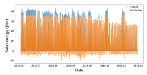
Figure 4: RNN testing curves of solar energy

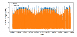
Figure 5: LSTM training curves of solar energy

Figure 6: LSTM testing curves of solar energy

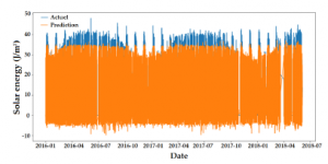
Figure 7: GRU training curves of solar energy

Besides, while RMSE is regarded in the literature as a good metric for evaluating and comparing regression models, it is still difficult to interpret properly. Therefore, we also normalize the RMSE values to provide a more meaningful representation of our results, which would allow more efficient conclusions. The normalized RMSE (NRMSE) represents the rate of the RMSE value and the range (the maximum value minus the minimum value) of the actual values. Table 3 shows a results synthesis based on this metric for real-time solar energy prediction. We can observe that RNN and

LSTM provide good and similar NRMSE values with 0.055 and 0.058 respectively.

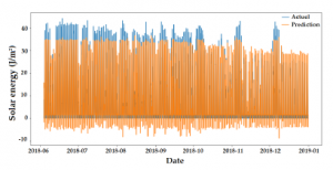
Figure 8: GRU testing curves of solar energy

Table 3: Results synthesis for real time prediction.

Models	Data	NRMSE
RNN	Training Test	0.055 0.066
LSTM	Training Test	0.058 0.068
GRU	Training Test	0.077 0.089

5. Conclusion and Perspectives

With the growing deployment of solar energy into modern grids, PV solar energy prediction has become increasingly important to deal with the volatility and uncertainty associated with solar power in these systems. In the literature, different models have been proposed for the prediction of PVs by using the AI techniques capacity. However, the majority of the research contributions in this area offer different techniques for making separate short-term and long-term forecasts, and do not focus on real-time forecasts. For this reason, we are working to find a model capable of producing continuous real-time forecasts using meteorological data, which is primordial for providing important decision support for power system operators to ensure more efficient management and secure operation of the grid and enhance the cost-effectiveness of the PV system. In this study, we investigated the efficiency of three different DL models: RNN, LSTM and GRU. The models were tested with data from a Moroccan region to make real-time PV forecasts. Further, the analysis of the results was based on six metrics MAE, MSE, RMSE, ME, R² and NRMSE to determine both forecast accuracy and margin of error. The results prove the efficiency of RNN and LSTM for real-time PV prediction thanks to their ability to address long-term dependencies in sequential information for time-series regression problems, compared to GRU that gives slightly less performance than the RNN and LSTM. From these findings, it can be concluded that RNN and LSTM showed very high accuracy and low errors, they are reliable models that can minimize errors in the learning and testing process, in addition to reduce the uncertainties associated with the operation and planning of integrated PV energy management systems. Moreover, they are promising techniques that also appears to be suitable for long-term PV forecasting and should be studied and recommended as a possible unified and standard tool for real-time, short-term and long-term PV prediction. As future work of this study, we plan to enhance these models by employing other approaches, extend them to longer term PV forecasting, as well as to studying other promising deep learning methods in view of providing and deploying a powerful model for PV energy prediction.

Conflict of Interest

The authors declare no conflict of interest.

1. E. Hache, “Do renewable energies improve energy security in the long run? Septembre 2016 Les cahiers de l’e´conomie – no109 Se´rie Recherche,” 2016.
2. M.G. De Giorgi, P.M. Congedo, M. Malvoni, “Photovoltaic power forecasting using statistical methods: Impact of weather data,” IET Science, Measurement and Technology, 8(3), 90–97, 2014. DOI:10.1049/iet-smt.2013.0135.
3. P. Li, K. Zhou, S. Yang, “Photovoltaic Power Forecasting: Models and Meth- ods,” 2nd IEEE Conference on Energy Internet and Energy System Integration, EI2 2018 – Proceedings, 1–6, 2018. DOI:10.1109/EI2.2018.8582674.
4. U.K. Das, K.S. Tey, M. Seyedmahmoudian, S. Mekhilef, M.Y.I. Idris, W. Van Deventer, B. Horan, A. Stojcevski, “Forecasting of photovoltaic power genera- tion and model optimization: A review,” Renewable and Sustainable Energy Reviews, 81(August 2017), 912–928, 2018 DOI:10.1016/j.rser.2017.08.017.
5. A. Youssef, M. El-telbany, A. Zekry, “The role of artificial intelligence in photo- voltaic systems design and control: A review,” Renewable and Sustainable En- ergy Reviews, 78(November), 72–79, 2017. DOI:10.1016/j.rser.2017.04.046.
6. A.P. Yadav, A. Kumar, L. Behera, “RNN Based Solar Radiation Forecasting Using Adaptive Learning Rate,” 442–452, 2013.
7. G. Li , H. Wang, S. Zhang, J. Xin, H. Liu,“Recurrent Neural Networks Based Photovoltaic Power Forecasting Approach,” 1–17, 2019.
8. P. Li, K. Zhou, X. Lu, S. Yang, “A hybrid deep learning model for short- term PV power forecasting,” Applied Energy, (November), 114216, 2019. DOI:10.1016/j.apenergy.2019.114216.
9. M. Abdel-Nasser, K. Mahmoud, “Accurate photovoltaic power forecasting models using deep LSTM-RNN,” Neural Computing and Applications, 31(7), 2727–2740, 2019. DOI:10.1007/s00521-017-3225-z.
10. H. Zhou, Y. Zhang, L. Yang, Q. Liu, K. Yan, Y. Du, “Short-Term Pho- tovoltaic Power Forecasting Based on Long Short Term Memory Neural Network and Attention Mechanism,” IEEE Access, 7, 78063–78074, 2019. DOI:10.1109/ACCESS.2019.2923006.
11. Y. Yu, J. Cao, J. Zhu, “An LSTM Short-Term Solar Irradiance Forecasting Under Complicated Weather Conditions,” IEEE Access, 7, 145651–145666, 2019. DOI:10.1109/ACCESS.2019.2946057.
12. J. Wojtkiewicz, M. Hosseini, R. Gottumukkala, T.L. Chambers, “Hour-Ahead Solar Irradiance Forecasting Using Multivariate Gated Recurrent Units,” 1–13, 2019. DOI:10.3390/en12214055.
13. M. Hosseini, S. Katragadda, J. Wojtkiewicz, R. Gottumukkala, “Direct Normal Irradiance Forecasting Using Multivariate Gated Recurrent Units,” 1–15, 2020. DOI:10.3390/en13153914.
14. K. Yan, H. Shen, L. Wang, H. Zhou, M. Xu, Y. Mo, “Short-Term Solar Irradi- ance Forecasting Based on a Hybrid Deep Learning Methodology,” 1–13.
15. M.Q. Raza, M. Nadarajah, C. Ekanayake, “On recent advances in PV out- put power forecast,” Solar Energy, 136(September 2019), 125–144, 2016. DOI:10.1016/j.solener.2016.06.073.
16. C. Wan, J. Zhao, Y. Song, Z. Xu, J. Lin, Z. Hu, “Photovoltaic and solar power forecasting for smart grid energy management,” CSEE Journal of Power and Energy Systems, 1(4), 38–46, 2016. DOI:10.17775/cseejpes.2015.00046.
17. A. Tuohy, J. Zack, S. E. Haupt, J. Sharp, M. Ahlstrom, S. Dise, E. Grimit, C. Mohrlen, M. Lange, M. G. Casado, J. Black, M. Marquis, C. Collier, ”Solar forecasting: Methods, challenges, and performance,” IEEE Power and Energy Magazine, 13(6), 50-59, 2015.DOI:10.1016/j.111799.
18. G. Notton, M.L. Nivet, C. Voyant, C. Paoli, C. Darras, F. Motte, A. Fouil- loy, “Intermittent and stochastic character of renewable energy sources: Consequences, cost of intermittence and benefit of forecasting,” Renew- able and Sustainable Energy Reviews, 87(December 2016), 96–105, 2018. DOI:10.1016/j.rser.2018.02.007.
19. A.A. Merrouni, F.E. Elalaoui, A. Mezrhab, A. Mezrhab, A. Ghennioui, “Large scale PV sites selection by combining GIS and Analytical Hier- archy Process. Case study: Eastern Morocco,” Renewable Energy, 2017. DOI:10.1016/j.renene.2017.10.044.
20. A. Alzahrani, P. Shamsi, C. Dagli, M. Ferdowsi, “Solar Irradiance Forecasting Using Deep Neural Networks,” Procedia Computer Science, 114, 304–313, 2017. DOI:10.1016/j.procs.2017.09.045.
21. A. Alzahrani, P. Shamsi, M. Ferdowsi, “Solar Irradiance Forecasting Using Deep Recurrent Neural Networks,” 5(1), 1-6, 2017.
22. Y. LeCun, Y. Bengio, G. Hinton. ”Deep learning.” Nature 521(7553), 436-444, 2015.
23. H. Wang, Z. Lei, X. Zhang, B. Zhou, J. Peng, “A review of deep learning for re- newable energy forecasting,” Energy Conversion and Management, 198(July), 111799, 2019. DOI:10.1016/j.enconman.2019.111799.
24. X. Qing, Y. Niu, “Hourly day-ahead solar irradiance prediction us- ing weather forecasts by LSTM,” Energy, 148, 461–468, 2018. DOI:10.1016/j.energy.2018.01.177.
25. H. Liu, X. Mi, Y. Li, “Comparison of two new intelligent wind speed forecast- ing approaches based on Wavelet Packet Decomposition , Complete Ensemble Empirical Mode Decomposition with Adaptive Noise and Arti fi cial Neural Networks,” Energy Conversion and Management, 155(July 2017), 188–200, 2018. DOI:10.1016/j.enconman.2017.10.085.
26. Y. Wang, W. Liao, Y. Chang, “Gated Recurrent Unit Network-Based Short- Term Photovoltaic Forecasting,” 1–14, 2018. DOI:10.3390/en11082163.
27. K. Cho, B. van Merrienboer, C. Gulcehre, F. Bougares, H. Schwenk, Y. Bengio, “Learning Phrase Representations using RNN Encoder–Decoder for Statistical Machine Translation,” 2014.
28. M. C. Sorkun, C. Paoli, O¨ . D. Incel, ”Time series forecasting on solar irradi- ation using deep learning,” 2017 10th International Conference on Electrical and Electronics Engineering (ELECO), Bursa, 151-155, 2017.
29. H.M. Lynn, S.B.U.M. Pan, “A Deep Bidirectional GRU Network Model for Bio- metric Electrocardiogram Classification Based on Recurrent Neural Networks,” IEEE Access, 7, 145395–145405, 2019. DOI:10.1109/ACCESS.2019.2939947.
30. Z. Che, S. Purushotham, K. Cho, D. Sontag, Y. Liu, “Recurrent Neural Net- works for Multivariate Time Series with Missing Values,” Scientific Reports, 1–12, 2018. DOI:10.1038/s41598-018-24271-9.
31. H. Zhou, Z. Deng, Y. Xia, M. Fu, “A new Sampling Method in Particle Filter Based on Pearson Correlation Coefficient,” Neurocomputing, 2016. DOI:10.1016/j.neucom.2016.07.036.
32. D.P. Kingma, J. Ba:, ”Adam: A Method for Stochastic Optimization,” Proceed- ings of the 3rd International Conference on Learning Representations (ICLR), p. No abs/1412.6980, 2014.
33. F. Wang, Z. Mi, S. Su, H. Zhao, “Short-term solar irradiance forecasting model based on artificial neural network using statistical feature parameters,” Energies, 5(5), 1355–1370, 2012. DOI:10.3390/en5051355.
34. B.J. Miles, “R Squared , Adjusted R Squared,” Wiley, 2014.
35. C. Onyutha, “From R-squared to coefficient of model accuracy for assessing ” goodness-of-fits ”,” (May), 2020.
36. D.B. Figueiredo Filho, J.A.S. Ju´nior, E.C. Rocha, ”What is R2 all about?,” Leviathan (Sa˜o Paulo), 3, 60–68, 2011.
37. I. Jebli, F. Belouadha, M.I. Kabbaj, “The forecasting of solar energy based on Machine Learning,” (c), 2020 International Conference on Electrical and Information Technologies (ICEIT). IEEE, 1-8, 2020.

(Click Here)

(Click Here)