1.Introduction

Education is a determining factor for growth and development and education systems and socio-economic development are closely related and interact with each other [1]. Indeed, an education system enables individuals to improve their productivity and increase their employability, and at the community level, it improves the competitiveness and attractiveness of the economy through the availability of skilled human capital. As a result, developing effective education systems whose performance can be quantified and ensured becomes an important issue at many levels for managers and all stakeholders.

But several questions arise: what defines an education system as a high-performing one? How can the performance of an education system be evaluated? What makes an education system efficient? What are the factors that impact its performance? How can we act on these factors to improve this performance?

Answers to these questions are not obvious as far as education systems are complex systems and having tools allowing the objective evaluation of their performance is still a goal to achieve due to the multidimensional and complex nature of these systems.

In [2]-[4], the authors have dealt with the reasons and some consequences of the complex nature of education systems and their nonlinear behavior.

This complexity is related to the existing interconnections between the different levels of educational systems starting from kindergarten to reach high schools and universities. Low performance at one level tends to affect the global performance at subsequent levels. Furthermore, individual’s performance in schools is influenced by several other systems. Education is in fact part of a larger system whose elements, such as economics, culture, society, and politics, interfere with it.

Education systems are also time-dependent and, changes in education often take a long time. Implemented policies may show results many years later, sometimes decades after their implementation. Another issue is that behaviors and actions of one part of the educational system tend to affect other parts of the system. This complexity can lead to unpredictable consequences of implemented actions. Effective management of education systems, therefore, requires a global approach that oversees the effect of all the parameters considered as a whole to ensure an efficient system operation.

Modelling can be one of the useful methods to evaluate performance and to identify the factors or areas of improvement of this performance. Modeling a system consists of designing a representation of this system for analysis and simulation purposes to answer questions. There can be several models for the same system with different levels of precision depending on the phenomena to be studied. Identification of the appropriate model will depend on the questioning under consideration [5].

The use of complex and dynamic systems modelling to social systems is quite recent and its pertinence in the case of an educational system is continually increasing [2]. The main challenge is to develop a model that can capture the dominant dynamics of these systems while being at the same time, simple enough to be useful for analyzing, simulating, and quantifying the impact of different parameters on the global performances of these systems

Several works have focused on the modelling of education systems. They concerned areas such as design, operations, analysis of performance, and management.

In the field of production engineering, studies on education systems modelling have focused on developing an analogy between education systems and systems of production of goods and services. Once this analogy was established, methods and methodologies for production systems modelling were applied to education systems while adapting them to the specificities of the latter. This works has enabled the transfer of business process modelling tools to the field of education and thus provided models for various purposes such as quality assurance, computerization of processes, or the design of new systems.

In this way, in [6], the author used the SADT method (Structured Analysis and Design Technique) for the analysis and the functional decomposition of a school using Le Moigne’s systemic approach. Based on CIMOSA (Computer Integrated Manufacturing Open Systems Architecture) and IDEF0 (Integrated Computer-Aided Manufacturing Definition), he proposed modelling of the skills production system and engineering design of this system.

In [7], a model for resource specification for the planning of training activities using UML (Unified Modelling Language) and a model of the business processes of an education system using MECI (Modélisation d’Entreprise pour la Conception Intégrée) are proposed.

In higher education, in [8], the author proposed a model for quality improvement by identifying the skills that graduates must acquire and proposes the activities and means to achieve this objective by using business process modelling BPM.

In relation to the increasing use of digital technologies, the author in [9] proposed a personalized training path per learner according to his/her individual capacity to optimize academic performance using Petri nets.

In [4], the author investigated the application of dynamic systems modelling for educational policy analysis to a better understanding of the dynamics of the current system and the design of evolution scenarios for the future. He applied this approach during a case study during the school year 2007-2008 in the American state of Rhode Island.

Another class concerns the demographic models used for the simulation of educational policies and strategies. This is the case of the EPSSIM code (Education Policy and Strategy Simulation Model) [10] which is a generic model designed by UNESCO. It provides technical and methodological support for the elaboration of educational development plans. It is a demographic model in which schooling objectives are considered as decision variables and expenditures are calculated as a consequence of the achievement of these objectives. It essentially allows the students flow simulation and costs calculations.

These models, which remain partial, can simulate the behavior of the system for a reduced number of basic quantitative parameters and require a high degree of granularity to ensure their operationality and reliability of their results

This paper aims to present an educational system model for studying the impact of various parameters on the behavior of the system and to estimate its performance. The focus will be on the study of the impact of learners’ competencies deficit on the performance of a training program.

2. Modelling of an education system

2.1. Modelling a training unit

A previous work [11], allowed us to propose a model of an education system that makes it possible to simulate its behavior to predict its long-term evolution, to evaluate its performance, and to simulate the impact of some factors on the evolution of this performance.

According to previous works which consider that an educational system can be defined as a competence production system [6] and also that any system which includes, even partially, in its missions the increase of learner skills can be considered as a part of an educational system [12], the approach conducted for the modelling of such system consists in proposing a decomposition of this system to introduce the notion of training unit which is the basis of the proposed modelling.

Despite the specificities of each country, educational systems at the global level are fairly homogenous and exhibit a quite similar central core. Therefore, most educational systems around the world have four educational levels: pre-primary, primary, secondary, and tertiary. The present simulation considers also that each training cycle, provided usually in an educational institution, can be further divided into training programs, with each program composed of a limited number of courses consisting of a defined number of sessions.

Similarly, to the goods or services production systems, educational systems have organizational units, these are the training units. A training unit aims to transform business object inputs (can be physical or informational) into business object outputs within a framework of objectives and constraints fixed by the external conduct rules of the unit. A training unit can correspond to different parts; it can be a whole educational system, a training cycle, a training institution, or even a single classroom session. Thus, the reconstruction of the global system can be done by grouping a range of training units in parallel and/or in series according to well-defined rules.

To model the training unit, we relied on models based on BPM tools and mainly the work related in [13] where the author suggests using a generic processor to characterize the activities of both the physical and decision systems to evaluate its performance. A generic processor is an entity that performs one or more basic transformation activities, and that fits into the structure, thus modifying its behavior and performance. By organizing a set of generic processors in a network, it creates a particular state of the production system which is characterized by a performance level.

Thus, the training unit is an entity of the training system with the objective to transform the inputs competencies’ level of the learners into a higher level of output competencies respecting the constraints and objectives of the educational system and thus to contributes to the achievement of the overall objectives of the training system. The reconstruction of the global system will then be reconstructed by grouping together a set of training units, either in parallel or in series according to well-defined rules.

Thus, the objective of a training unit is to increase the level of competencies of learners starting from an input reference competency C_r, to a level above an output reference competency C’_r on a fixed time h, by using resources and based on conduct and achievement data as shown in Figure 1.

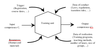Figure 1: Model of a training unit

Educational systems present a particularity insofar as learners are co-producers of the service they use. In fact, each student has his own sensitivity to the process of skills acquisition. The objectives to be achieved by a training unit are defined during the design of this training unit. In this way, the reference input competencies needed to correctly follow this training activity, the reference output competencies to be reached, the resources required to carry out the activity, the conduct of data, and the achievement data are defined.

The interest of this modelling lies in the possibility of decomposing or aggregating the education system into networks of generic processors of different levels and by extension the possibility of evaluating the global or detailed performance of the training system on any level of abstraction.

The educational system is modeled as a series of training units interacting with each other to produce the targeted competencies.

Figure 2: reconstitution of training units into a training program

Figure 2 illustrates an example of aggregating a set of training units by levels to reconstruct a training program. Each level groups together a defined set of training units and each training unit aims to achieve a defined increase in learner’s competencies. Resources to be mobilized for a training unit to carry out its activity are defined, as well as related data of realization, data of conduct, and the launcher of the activity of the processor. The rules relating to the access of a learner from one level to the next level are also fixed, thus determining the time evolution of the training program.

This model allows the identification of what the training unit does, its function, as well as the determining factors for its functioning. Subsequently, the current modelling is associated with a simulation model which is built on the educational production function [14] and the learner’s theories’ results [15] in order to simulate the behavior of the system over time and the effect of some factors on its performance in a quantitative manner.

2.2. Mathematical model a training unit

The training unit is associated with a mathematical model based on the educational production function, that is written in a general form as follows [14]:

                                        A = f*(X1, …, Xn)                                  (1)

where A is some measure of output, expressed as a function of a set of variables X1…..Xn.

In [11], the output A was the increase of competence level of a learner, noted as ΔC_i, while the parameters X_i that will be taken into consideration, at first approximation, are the duration of the training unit, the personal capacity of each learner µ_i, the input competence which represents the characteristics of the learners, the class size and a score for the pedagogical methods which represent some parameters of the resources and the data of conduct. The other parameters remain constant throughout the simulation and therefore they will not impact the variation of ΔC_i.

Thus, expression (1) may be expressed as follows:

                                        ΔC_i = f(h, µ_i, k, g)                                   (2)

where ΔC_i is the competence level’s increase of the learner i, h the training unit’s duration, µ_i the individual capacity of competence acquisition of the learner i, k the coefficient representing the gap between the input competence of learner i and the required input competence of the training unit; g the coefficient taking into account the effect of the class size and the pedagogical methods.

An approach to specifying the function f and the relation linking the parameters h, µ_i, and g to the output ΔC_i to carry simulations is presented in previous work [11].

      Expression (2) becomes as follows:

Where C’_r is the output competence’s reference, C_r is the input competence’s reference, h the training unit’s real duration, h_r the training unit’s reference duration, α a parameter characterizing the progressivity of the evolution of the level of competence during the training.

The coefficient μ_i, which is specific to each learner, expresses his ability to achieve the expected competencies with more difficulty (μ_i<1) or more ease (μ_i> 1) than was projected in the design of training. The reference value for μ_r is 1.

For the coefficient g, we assume, in a first approximation, that a change in excess (resp. in default) of the class size is not beneficial (resp. beneficial) to the learner, so we can use a linear relation to model this coefficient as follows:

                                       g(n) = b if n > n_max

                      g(n) = b+((a-b)/2)*n if  n_min <n< n_max                  (4)

                                       g(n) = a if n < n_min

where n is the ratio of the number of students in the group to the number recommended by the pedagogical method, a and b are the maximum and minimum values taken by the function g(n) when the group size is above a value n_max or below n_min.

Note that for the simulation results that will be presented here, we have used another relation instead of (4), which seems more adapted even if it presents similar characteristics, it is given by:

A possible lack of the input competence C_i is taken into consideration through a factor k(C_i/C_r) which reflects the difference between the learner’s input competence C_i and the reference input competence C_r required by the training unit.

2.3. Performance of a training unit and a training program

Following [11], performance can be defined as the ratio of the actual result obtained as process output to an expected result under standard conditions to be defined.

The training unit’s result is determined as all competence increases accomplished by the students and validated following the outbound validation rules.

The expected standard result can be considered as the sum of the increases in the levels of competencies that are assumed to be validated by the learners when all the parameters of the production function of the training unit defined by relation (3) are taken equal to the reference values of the parameters.

Therefore, the training unit performance can be expressed as follows:

where P is the performance of the training unit, (C’_i – C_i) the competence level increase of learner i having successfully validated the training unit, n is the number of learners who validate the unit, and (C’_r-C_r)*n_r is the expected increase in the competence level of the class when all parameters are equal to their reference values.

A training program is considered as a network of interconnected training units distributed by the level of training with rules for transition from one level to another. The training units of a training level are connected in parallel and form a block and each training unit performs a defined competence increase activity. Thus, a training program that consists of n blocks, each block consisting of k training units, is schematized by a network of m processors such that m=n*k. The training units are denoted U_ij where i (1 … n) denotes the number of the block to which it belongs and j (1 … k) its classification within the block.

To define the performance of the training program, the performance of the training blocks making up the training program must first be defined.

We can then define the performance of block i of training units P_i as follows:

where   is the sum of all the increases in competencies of the learners who have validated the training units that constitute the training block,  is the sum of all the increases in competencies expected by the training units when the other parameters values are those of the reference data.

The performance of the training program can be calculated as the average performance of the training blocks weighted by the respective numbers of learners and can be translated by the following expression:

where, P_i is the performance of training block i, g_i is the overall number of learners in block i, and n the number of blocks in the training program.

Thus, a model based on a mathematical formulation and a numerical simulation is obtained, it allows the calculation of the performance of a training program, based on the performance of the training units constituting this program. The effects on the overall performance of the training program of the variation of different parameters can thus be simulated and quantified.

This model was used in [11] to show the effects of the individual capacity of the learner’s competence acquisition, as well as the pedagogical method’s sensitivity in association with the group’s size on the performance of a training unit.

The objective of this paper is to analyze the effect of the learner input competencies deficit factor on the behavior of a training unit and its performance and also to extend the approach to the case of a training program.

3. Impact of the input competence factor: results and discussion

For the chosen model, the education system is approached as an organized whole for skills production, composed of training units linked in parallel, and series according to rules of arrangement. Each unit has its own training objective, which is to increase specific skills of learners from a given level of competence at the input, assumed to be achieved by all entrants to the unit, to a higher level of competence at the output. The specificity of such a system is that the learners are co-producers of the service they use, which means that their characteristics will influence this increase in competencies. In fact, not all entrants to training have reached the required input level of competence and do not also have the same aptitudes for the acquisition of new skills.

Several studies have shown the important role of the learner in the process of competencies acquisition [16]-[18].

In a study using a multilevel model to identify the most important variables affecting students’ performance [16], the authors have found evidence that both the students’ and their families’ characteristics play a role in the former’s performance.

As stated in [19], precedent results and skills already acquired are strongly linked to the ease with which students will develop new skills, and thus have a real effect on their academic performance. In [20] and [21], the authors highlighted the importance of prior knowledge for success in studies.

In previous works [11], the personal characteristics of the learners are incorporated into the model through two factors. The first factor is the “personal capacity for competence acquisition µ_i” factor, which is specific to each learner and for each training unit and which is dedicated to taking into account the specific aptitudes of a learner allowing him to more easily assimilate new content. The impact of this factor on the increase in competencies and on the performance of a training unit was analyzed.

The second factor is the learner’s prior knowledge through a “k” factor which quantifies the inadequacy between the student’s input competence and the competencies entry level required by the training unit. In what follows, we will focus on the role of the latter, by establishing the effect of the factor k on the development of student’s competence, on the training unit’s performance, and on the training program’s performance.

3.1. Evolution law of the coefficient k(C_i/C_r)

The goal sought is to establish an expression of the factor k which includes in the model defined by equation (3) the fact that a learner who would have a lack of competence at the entry of the training unit is less efficient in achieving the expected skills increase during the training. For that, we introduce the following expression:

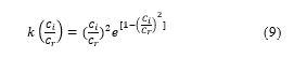Equation (9) allows a variation of the coefficient k between the values 0 and 1, with k = 0 when C_i = 0 and k = 1 for C_i = C_r. This reflects the fact that a learner with a zero value of input competence, cannot progress through the training, and a learner who has required competence at the entry should achieve the expected level of competence at the output. While if a learner has achieved a level of competence C_i above the reference input level C_r, the benefit of training is less and allows only a small increase of competence.

The graph below shows the evolution of the factor k as a function of the ratio C_i/C_r.

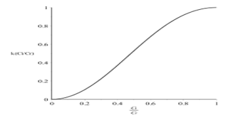Figure 3: Evolution of the coefficient k as defined to the expression (9)

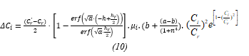
The mathematical model of the training unit (3), coupled to (9), is then given by the following expression:

We will therefore consider three situations for the simulations. The first one shows the effect of the input competence on the competence increase’s evolution, the second simulation concerns the effect of this factor on the training unit’s performance and the third simulation reveals the effect of this factor associated with other factors on the training program’s performance.

3.2. Simulation on the evolution of the increase of competence

The simulations to be carried out aim to determine the effect of the learners’ skill level at the beginning of a training course on the progression of skills acquisition during the training process.

To illustrate this impact, we consider three groups of learners, the first group identified by a level of skills C_i below the required reference level C_r, the second having a skills level C_i equal to the required level, and the third having a level above the required level.

For the three groups, we consider all the other parameters of the simulation set to their reference values i.e. the training hours’ number performed h is consistent regarding the reference duration of the training unit h_r (h = h_r), the students have a competence acquisition capacity μ_i = μ_r and the coefficient g(n) is equal to 1.

Expression (10) above then allow simulation of the increase of competence in each of the three cases

Figure 4: Input competence’s effect on the competence increase

Figure 4 shows the input competence’s effect on competence increase. The learner who starts the training with a deficit of competence’s input (curve point), will not reach the expected competence’s output. On the opposite, a learner with a competence’s input greater than the required level accomplishes an output competence higher than the expected reference competence.

These results are in concordance with the studies [19], [20] and [21] that establish links between preceding results and skills previously acquired by the learners and the ease with which they acquire new skills

3.3. Simulation of the input competence’s effect on the performance of a training unit

The goal set here is to simulate the effect of the variation in the input competence factor “k” on a training unit performance. Given the particularity of the educational systems in which every learner is a co-producer of his own competence increase according to his individual capacity of acquiring competencies µi, this factor is introduced in the following simulations.

Since the purpose is to focus on the input competence factor’s variation, the other parameters are set to their reference values for the training unit, namely (C_r, C’_r, h_r, n_r) as well as the training unit validation’s rule that defines the minimum value of ΔC that the learner must reach to validate the training unit.

To realize the simulation, we consider, for a training unit, the following parameters reference values. The reference values are C_r=50 for the input competence, C’_r =100 for the output competence, h_r = 50 for the training unit duration, and n_r = 100 for the learner’s number. We also consider that learner i validate the training unit if (C’_i – C_i)³(C’_r – C_r). The simulation of the effect of the input competence on the training unit performance is executed according to the algorithm illustrated in Figure (5).

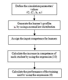Figure 5: The simulation’s algorithm

The first step for the simulation is to define the simulation parameter’s values, the used values are n_r=100, C_r =50, C’_r =100 and h_r =50, and the training unit validation’s rule that determine the minimum value required for ΔC_i that the learner has to reach in order to validate the unit. The second step is the generation of the student’s profiles by using a normal law distribution for the parameter µ_i. The third step consists, for every simulation, in assigning the input competence C_i for the students. The fourth step is the calculation by relation (10) of the increase in competence for each learner. In the end, we calculate the performance of the training using relation (6).

Four simulations are carried out by varying the learners’ input competence. In the first case, the input competence of learner’s C_i is equal to the reference input competence of the training unit C_r, In the second case, the C_i deficit is of -3% compared to C_r, for the third case the C_i deficit is of -5% compared to C_r and the for the last case the C_i deficit of -7% compared to C_r.

The simulations’ results are illustrated in the graph below:

Figure 6: Impact of the input competence deficit on the performance of a training unit

These results highlight the effect of the deficit of learners’ input competencies on the training unit performance.

We note that when all learners have the required input competence to follow the training unit, i.e. C_i=C_r, the performance of the training unit is around 59%. This percentage is consistent and is due to the distribution in normal law retained for the personal capacity of competence acquisition µ_i, which is an essential factor of the learner. If these learners have an input competence deficit of -3% compared to the reference input competence, then this performance decreases and becomes of the order of 36%. Therefore, the improvement of a training unit performance, requires to check the input competence of a learner, so that the follow up of the competence acquisition process can be done properly.

3.4. Simulation of the impact of the input competence on the performance of a program training

The purpose is the stimulation of the input competence’s impact and other parameters as the individual capacity of competence acquisition µ_i the class size on the performance of a training program and monitor its behavior over time.

 The organization of the training program is illustrated by the following figure:

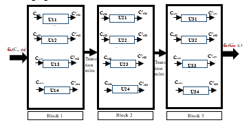Figure 7: Organization of a training program

The training program for the simulation consists of three training blocks and each training block consists of four training units. The data of the realization of the training units are given in Table1.

Table 1: Training unit realization data and mobilized resources initialized to reference data

Level of training 1	Reference input competence	Reference output competence	Reference duration	Reference group size	Number of hours realized	Real group size	Number of groups
U 11	50	100	50	25	50	25	2
U 12	50	100	50	25	50	25	2
U 13 U 14	50 50	100 100	50 50	25 25	50 50	25 25	2 2
Level of training 2	Reference input competence	Reference output competence	Reference duration	Reference group size	Number of hours realized	Real group size	Number of groups
U 21	100	150	50	20	50	20	2
U 22	100	150	50	20	50	20	2
U 23 U 24	100 100	150 150	50 50	20 20	50 50	20 20	2 2
Level of training 3	Reference input competence	Reference output competence	Reference duration	Reference group size	Number of hours realized	Real group size	Number of groups
U 31	150	200	50	15	50	15	2
U 32	150	200	50	15	50	15	2
U 33 U 34	150 150	200 200	50 50	15 15	50 50	15 15	2 2

For the simulation, we consider that 100 learners are enrolled per year for level 1, 80 for level 2, and 60 for level 3.

The algorithm in Figure 8 illustrates how the simulation is performed

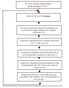Figure 8: Algorithm for simulating the performance of a training program

The simulation is performed for seven iterations up to Year 7 of the training program. The objective is to track the behavior of the variation in performance over the seven years of training. The simulation is carried out with a constant number of new learners NI entering Level 1 for each year of study.

Figure 9 below is an illustration of the simulation’s result.

Figure 9: Simulation of the performance of a training program with NI constant

Figure 9 illustrates the variation in the performance of the training program on three different curves. The first curve (Curve A with continuous line) represents the impact of the personal capacity of competence acquisition µ_i. In this case, the coefficients of the group size g(n) and the input competencies k(C_i/C_r) are kept equal to 1. The second curve (curve B with dashed line) represents the impact of the personal capacity of competence acquisition µ_i and the coefficient of the group size g(n). The factor of the input competencies k(C_i/C_r) is kept equal to 1. The third curve (Curve C with dotted line) reflects the impact of the personal capacity of competence acquisition µ_i, the coefficient of group size g(n), and the input skills factor k(C_i/C_r).

For curve (A), in the first year of the training program, the performance of the training program is close to 50%. This is due only to the impact of the learners’ µ_i factors, which are distributed according to a normal distribution whose average is 1. Thus, nearly 50% of the learners have a µ_i factor less than 1 and therefore cannot reach the required output competencies. For year 2 this performance increases to nearly 80%. This is explained by the fact that the learners who move up to the higher levels in year 2 satisfy the required input competencies and their µ_i are greater than or equal to 1, which allows them to reach the output competencies. Moreover, for learners at the different levels who fail and repeat some training units, they validate these units since they have re-enrolled with their output competencies from year 1 as input competencies for year 2 that are higher than the required competencies, thus making up for their µ_i deficit. The 20% performance deficit is mainly due to the new learners who enrolled in level 1, 50% of whom have a µ_i<1 factor. Beyond this year, performance stabilizes at just over 80%. Thus, under the conditions of this simulation, i.e., without considering the effects of group size and the deficit in the input competence, the impact of the µ_i factors is offset by the increase in competencies of learners with a µ_i<1 for the second enrolment in the same training unit.

For curve (B), in addition to the impact of µ_i, the impact of the group size is included. By comparing curve (A) and curve (B), the impact of group size is clearly apparent with a decrease in the performance of Year 2 of the training program. In fact, only µ_i has an impact on the performance of year 1. Thus, learners with a µ_i <1 in year 1 are re-enrolled in the same training units in year 2, thus increasing the group size of these training units and consequently this year’s performance is impacted by this increase in the number of learners. From year 3 onwards, performance increases and then stabilizes at the end of year 5. This is due, on the one hand, to the increase in the input competencies of learners who repeat a given level, which partially compensates for the impact of µ_i and group size, and, on the other hand, to the stabilized number of learners in the higher levels.

For curve (C), in addition to the impact of µ_i and group size, the impact of learners’ input competencies is included. Comparing this curve with the other two curves, we see that the factor of learner input competencies negatively affects the performance of the training program which stabilizes at the end of year 7 at a rate of 40%.

The results of this simulation allow us to compare and visualize the behavior and variation in the performance of a training program under the effect of the different simulation factors. These results also make it possible to quantify this variation in performance. Indeed, by acting on the learners’ input competencies through specific training actions for their improvement, the performance of the training program can be improved and go from a rate of 40% to a rate of nearly 80%. If we also act on the size of the group, performance can be further improved. Another performance improvement lever lies in the improvement of the learners’ personal capacity to acquire competencies. This simulation is carried out with a constant number of new learners who enroll in the training program each year.

Another simulation is carried out to study the effect of a change in the number of new registrants at the start of the program in year 1. We will consider three situations, the one for which the number of entrants is 100, then the one where this number is increased by 20% then the one where it is decreased by 20%

The results of this simulation are shown in the following graph:

Figure 10: Simulation of the performance of a training program with variable NI

Figure 10 illustrates the variation in the performance of the training program along three different curves. The first curve (curve A with a continuous line) represents the impact of the personal capacity of competence acquisition µ_i and the group size with the new number of learners conforming to the reference number of the block of level 1. The factor of the input competence k(C_i/C_r) is kept equal to 1. This curve corresponds to curve B of the previous simulation. This curve is considered as the reference curve for this simulation. The second curve (curve B with a dashed line) represents the impact of the µ_i and the coefficient of the group size g(n) with a number of new learners at the entrance 20% lower than the reference number. The factor of the input competence k(C_i/C_r) is kept equal to 1 and, the third curve (curve C with dotted line) represents the impact of µ_i, the coefficient of the group size g(n) with a number of new entrants 20% higher than the reference number. The factor of the input competence k(C_i/C_r) is kept equal to 1.

The performance of the training program in the start-up year “Year 1” varies according to the number of learners at the entrance. When the number of new entrants is reduced (curve B), the group size factor g(n) becomes greater than 1, which compensates for the effect of µ_i and therefore the performance of the training program increases, whereas when the number of new entrants is increased (curve C), the group size factor g(n) becomes less than 1, which contributes to the impact of µ_i in reducing the performance of the training program.

Whereas in the second “Year 2”, the results are reversed. Indeed, in the case of curve B, given the number of learners who validated in year 1, the group size of the different blocks in year 2 increased and consequently g(n) becomes less than 1 and impacts the increase in learners’ competencies and subsequently performance. The performance follows the same behavior until year 5, after which the performance increases, stabilizes, and approaches the performance of curve 1.

As for the behavior of the performance in the case of curve C, it follows the opposite behavior than that of curve B and in the stabilization phase, from year 5 onwards, the performance stabilizes at a rate of 60%, i.e. a decrease of 10% compared to the reference curve A.

These simulations on the performance of a training program illustrate the impact of the factors selected on this performance and make it possible to estimate, in a quantitative manner, the effects of variations in these factors on performance taken separately or in combination. The results of these simulations provide a better understanding of the interaction between the parameters and their impact on performance and can be used to test solutions for performance improvement.

4. Conclusion

By viewing education systems as skills production systems and by applying Business Processing Modelling methods, a modelling of education systems is proposed in the present work. The breakdown of the whole system allows us to introduce the training unit concept and then to organize these units in networks with units connected in series and parallel.

The objective of each training unit is to transform the learners’ level of competencies into higher-level output competencies while respecting the objectives and constraints set by the educational system. Each training unit thus contributes to the achievement of the general objectives of the training system. This is achieved by mobilizing resources and according to rules of realization and rules of conduct.

      Thus, the model proposed for the training unit has made it possible to determine the key factors influencing its performance. This model was coupled with a simulation model that allows to study the impact of the variation of these factors on the evolution of the system’s behavior and performance and to simulate this impact.

The presented results of simulations show the effects of the learners’ input competence deficit on the evolution of the process of competence increase and consequently on the performance of the training unit. Thereafter, the impact on the overall performance of a training program of this factor cumulated with those of the factors of the learners’ personal capacity to acquire competencies, and the group size is studied.

This modelling allows us to evaluate the performance of the training unit and the training program in a quantitative way and to simulate the behavior of this performance by varying the different factors. This modelling enables us to test solutions for performance improvement.

Let us note that a validation of the model on case studies remains to be carried out and will require in particular the establishment of strategies for identifying the various parameters involved in the laws introduced to characterize the learner’s aptitudes.

1. T. McCowan, “The Role of Education in Development,” Higher Education for and beyond the Sustainable Development Goals, Palgrave Studies in Global Higher Education, 2019, https://doi.org/10.1007/978-3-030-19597-7_2
2. N. Ghaffarzadegan, R. Larson and J. Hawley, “Education as a Complex System,” System Research and Behavioral Science, Wiley Online Library, 2016, DOI: 10.1002/sres.2405.
3. M. Koopmans, D. Stamovlasis, Complex Dynamical Systems in Education: Concepts, Methods, and Application, Springer, 2016. DOI 10.1007/978-3-319-27577-2
4. J. Groff, “Dynamic systems modeling in educational system: Design & Policy,” New approaches in educational research, 2(2), 72-81, 2013. DOI: 10.7821/naer.2.2.72-81
5. F.B. Vernadat, “Techniques de modélisation en entreprise : Application aux processus opérationnels, ” Economia, 1999.
6. C. Clementz, Modélisation des systèmes de production de compétences: apports à l’ingénierie pédagogique, Ph. D Thesis, Université de Metz, 2000. https://hal.univ-lorraine.fr/tel-01775474
7. O. Bistorin, Méthodes et outils d’aide à la conception des processus opérationnels des systèmes de formation, Ph. D Thesis, Université Paul Verlaine de METZ, 2007. https://tel.archives-ouvertes.fr/tel-01749013
8. M. Dragna et D. Ivanaa, “Business Process Modeling in Higher Education Institutions. Developing a Framework for Total Quality Management at Institutional Level,” Procedia Economics and Finance, 16, 95-103, 2014. doi: 10.1016/S2212-5671(14)00779-5
9. P. SeungSoon, “Applying Petri nets to model customized learning and cooperative learning with competency,” International journal computer science and network security, 8(2), 2008. DOI: 10.15693/ijaist/2016.v53i53.6-12
10. UNESCO, “Education, Policy & Strategy: Simulation Model EPSSim Version 2.1.” 2005.
11. N. Messaoudi, J. Khalid Naciri and B. Bensassi, “Simulating effect of parameter variation on the performance of an educational system,” International Journal of Simulation and Process Modeling, 13(3), 189-199, 2018. DOI: 10.1504/IJSPM.2018.10014176
12. O. Bistorin, C. Pourcel and P. Padilla, “Integrated model for operational process design of learning system,” 8e Conférence Internationale de MOdélisation et SIMulation, Hammamet, 2010.
13. H. Kromm, J. Deschamps, and G. Doumeingts, “Modélisation de processus pour une évaluation par niveaux de détail successifs, ” in 3e Conférence Francophone de Modélisation et de Simulation MOSIM’01, 2001.
14. S. Bowles, Towards an educational production function, National Bureau of Economic Research, 1970. http://www.nber.org/chapters/c3276.pdf
15. M. Benko, “On the Status of the Model of Growth of Knowledge by Repetition on the Field of Didactics,” Nitra, 2013.
16. F. Mourji and A. Abbaia, “Les déterminants du rendement scolaire en mathématiques chez les élèves de l’enseignement secondaire collégial au Maroc : une analyse multiniveaux,” Revue d’économie du développement, 21(1), 127–158, 2013. DOI : 10.3917/edd.271.0127
17. J.D. Williams and M.Somers, “Family, classroom, and school effects on children’s educational outcomes in Latin America,” School Effectiveness and School Improvement, 12(4), 409–445, 2001. DOI: 10.1076/sesi.12.4.409.3445
18. R.M. Felder and R. Brent, “Understanding student differences,” Journal of Engineering Education, 94(1), 57–72, 2005. DOI: 10.1002/j.2168-9830.2005.tb00829.x
19. R. J. Marzano, Building background knowledge for academic achievement, Alexandria: Association for supervision and curriculum development, 2004. ISBN 0-87120-972
20. D. Muijs and D. Reynolds, “Student background and teacher effects on achievement and attainment in mathematics: A longitudinal study,” Educational research and evaluation, 9(3), 289-314, 2003. https://doi.org/10.1076/edre.9.3.289.15571
21. B. Hemmings, P. Grootenboer and R. Kay, “Predicting mathematics achievement: the influence of prior achievement and attitudes,” International Journal of Science and Mathematics Education, 9(3), 691-705, 2011. https://doi.org/10.1007/s10763-010-9224-5

(Click Here)

(Click Here)