1.Introduction

Today, most of the information on the Internet is in the form of images, which may contain confidential information, such as patients’ medical records. In daily life, clinics or public health centers sometimes find it difficult to determine patients’ disease, and they need the help of hospitals or more experienced medical experts for analysis and diagnosis. Therefore, images of patients’ medical records must be sent from the clinic/public health center to the destination hospital. The problem is patients’ medical records are confidential and contains sensitive data. There are also regulations and legal protection of medical records. For example, Indonesia’s medical records regulation can be seen in [1]. So there has to be a way to maintain the security of patients’ medical records, which can be done by performing image encryption [2].

Basically, image encryption is a technique that is performed with the aim of protecting the content conveyed therein. This encryption is done by transforming the image into another form so that it does not contain meaningful information and cannot be understood visually or statistically. In general, there are two types of image encryption: traditional encryption and chaos-based encryption. Traditional encryption uses common encryption algorithms, such as the Data Encryption Standard (DES), International Data Encryption Algorithm (IDEA), or Advanced Encryption Standard (AES). Chaos-based encryption uses a sequence of (pseudo-)random numbers called chaotic maps as a key for encrypting images. Of these two types, chaos-based encryption is more suitable for use with images because the image consists of information (i.e., image pixels) with high redundancy and correlation, and the resulting encrypted image will be random and have low correlation between pixels. In contrast, traditionally encrypted images have more patterns, so they are more vulnerable to attack. In this study, two chaotic map models will be used: Arnold’s cat map for confusion or shuffling pixel positions and the Henon map for diffusion or changing gray values [3, 4].

To generate a chaotic map, there are several parameters that can be described as the key to the encryption and decryption process in this system. The generated chaotic map is influenced by these values, so the encryption and decryption process must use exactly the same parameter values. The slightest change to this value will result in a different output matrix, so there must be a mechanism that ensures the encryption and decryption process uses the same parameter values. In [4], author use the shared-key cryptography with Diffie-Hellman method to secure the key exchange process [5].

2.Literature Review

Chaos-based image encryption, commonly known as a chaotic system, is an approach to encrypting an image that involves chaotic maps, which are rows of random numbers generated by a mathematical calculation with certain initial values. This system is widely used in image encryption for several reasons: (1) it sensitive to initial values, (2) the resulting numbers are random, and (3) there are no patterns in the random number sequence, so it is difficult to predict [3, 6].

In general, there are two techniques that can be performed with chaos-based image encryption: confusion and diffusion. [6] Confusion involves shuffling the pixel positions that make up an image, while diffusion involves changing pixels’ gray values. In encryption, both techniques should be used; the use of just one can reduce the power of the encryption.           In [7], the author used chaotic system, the chaotic map plays a major role in both the confusion and diffusion processes. One of the chaotic map models that can be used for confusion is Arnold’s cat map (ACM), and one of the chaotic map models that can be used for diffusion is the Henon map, which is a mathematical model of the discrete-time dynamic system.

2.1. Arnold’s Cat Map

ACM is a chaotic map model that is used to randomize the pixel positions in an image. It was first introduced by Vladimir Arnold as a way to shuffle an image of a cat. Mathematically, this concept works by stretching and distorting a square shape and then reassembling it into the same shape [8, 9].

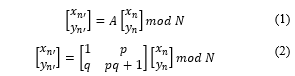
Since it was introduced, ACM has been intended to randomize the pixel position of an image so that it does not look the same, which is a confusion technique. ACM works by scrambling a pixel’s position without changing the value of the pixel itself. This can be done using the following formula [8,9]:

Although ACM is a chaotic map, if iterations are repeated many times, it is possible that the original image will be rearranged because the ACM concept relies on position randomization only. According to researchers, up to 3N iterations may be needed to return to the original image, where N is the dimension of the image [10].

Arnold’s cat map is commonly used for image encryption by shuffling the image pixels but actually it can be used to encrypt other form of multimedia data. In [11] and [12], there are good examples of audio encryption using Arnold’s cat map for securing voice communication. Arnold’s cat map can also be used to watermark an image or video, which is useful for tamper detection. In [13] and [14], there are some good examples of image watermarking, and [15] for video watermarking using Arnold’s cat map.

2.2. Henon Map

The Henon map is one of the most commonly studied discrete-time dynamic system models, and it has chaotic properties. It was first introduced as a simplification of the Lorenz model. It is formed by using a point (x_n, y_n) to map the next point using the following equation [16].

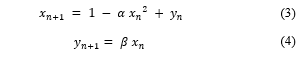In equations (3) and (4), x_n and y_n are the current point positions, while x_n+1 and y_n+1 are the next point positions. In the initial conditions, the values of x_n and y_n become initial values that will determine the next points. The slightest change in x_n and y_n in the initial conditions can have a big impact on the map that is formed [4, 17, 18].

The classic Henon map uses values of  = 1.4 and  = 0.3, which causes the results to be chaotic. Changes in both values can result in changes in the nature of the resulting map, which may not even be chaotic anymore [17, 18].

In image encryption, the Henon map model is often applied as a key stream generator for diffusion techniques or changing pixel values in images. To create this chaotic map, two initial values are needed, namely, the initial x and y values (x₀ and y₀). These are the key to establishing chaotic maps that will be used in both encryption and decryption processes [4, 17, 18].

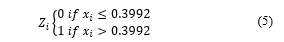
Chaotic maps are formed by calculating the Henon map formula with  iterations  represents the dimensions of the image, and  represents the number of bits in each pixel. For each iteration, a new  and  value is obtained and then converted to a bit value (0 or 1) using a threshold value which will later be converted to gray values for each pixel until the chaotic map is sized . In [18] Previous research [19] concluded that the cut-off value should be set at 0.3992 so that the sequence of numbers produced using the Henon map will be balanced. Thus, the decimal value x_n obtained at each iteration will be converted into binary form using a threshold value of 0.3992 based on the following equation:

2.3. Diffie–Hellman Key Exchange

The Diffie–Hellman key exchange (DH) is a method created for safe key exchange through public channels. It addresses the challenges that exist in a symmetrical cryptographic system, which uses only one key for encryption and decryption. Without using this method, key exchanges on symmetric cryptographic systems are performed outside the system, generally conventionally, to avoid key exchanges via public channels such as the Internet. [20]

DH offers the possibility of using both public and private keys for actual key exchange. The two keys are not related to the encryption process that will be carried out, but only serve to produce the actual key. Each client has a private key that only they known. From this private key, a public key can be generated through equation (6) [5, 20]:

where p is the prime value and g is the value of the agreed-upon generator. The resulting public key can be given to other people because it plays a role in creating a secret key for the two clients. To produce this secret key, the sender must perform a mathematical computation involving their private key and the recipient’s public key using equation (7) [5, 20]:

Likewise, when the recipient engages in decryption, the recipient must compute their private key and sender’s public key to produce a secret key that will be used in the encryption process. [20]

3. Proposed Model

In general, the system involves three parts: sender, receiver, and server. However, the implementation in this research only covers the client side; server settings have not been determined. The sending and receiving client side is where the Chaos-Based Image Encryption Program was run. The clinic/public health center, as the sending client, performs the encryption function, and the hospital, as the receiving client, performs the decryption function. The architecture of the whole system can be seen in Figure 1.

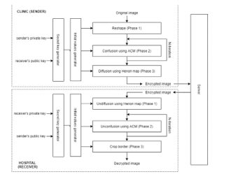Figure 1: Encryption and decryption architecture

According to this architecture, in order to carry out encryption and decryption, two types of inputs are required: keys and images. Two keys—a private key and a public key—are needed to produce a secret key that will be converted into initial values when making the chaotic map. After the image is encrypted, the image will be saved to the server so that it can be retrieved by the receiver for decryption. There are three stages of encryption: reshaping, confusion, and diffusion. Likewise, there are three stages of decryption: undiffusion, unconfusion, and crop border.

This research uses chaos-based encryption with a combination of confusion and diffusion methods. The choice of chaos-based image encryption is based on the nature of the image, which contains information (i.e., pixels) that have a high degree of redundancy and correlation with each other. By applying this type of encryption, the resulting image will be random, so it will have low redundancy and correlation between pixels. Another factor that reinforces the choice of chaos-based encryption is the nature of the chaotic maps we used, which are sensitive to changes in initial values ​​or parameters. A slight change in the initial values ​​will result in chaotic maps or rows of random numbers that have significant differences. This phenomenon is commonly referred to as the butterfly effect. Thus, this type of encryption is used to overcome statistical analysis attacks, which is more difficult with chaotic-based encryption results because of the randomness of the pixels making up the encrypted image [3, 21].

The combined use of confusion and diffusion is based on the nature of confusion, which shuffles pixels but does not change their values. This makes the image unrecognizable but still vulnerable to most attacks. Therefore, we used diffusion to change the pixel values of the randomized image. By using a combination of confusion and diffusion, the encryption results become more random and difficult to predict. In this encryption system, different chaotic maps are used for confusion and diffusion; Arnold’s cat map is used for confusion, while the Henon map is used for diffusion. This is done to increase resistance to attacks because each method uses a different mathematical model. In addition, we chose them because they have many dimensions and are both two-dimensional chaotic maps [21].

The encryption system designed and developed in this research is based on several previous studies. Eko Hariyanto and Robbi Rahim previously explained the use of Arnold’s cat map to encrypt images using the confusion technique in a study entitled “Arnold’s Cat Map Algorithm in Digital Image Encryption.” In [9], author explained how Henon maps could be used to encrypt images by applying a combination of confusion and diffusion in a study entitled “A Chaotic Confusion-Diffusion Image Encryption Based on Henon Map” [22]. In addition, the author described the use of Arnold’s cat map and the Henon map to encrypt images in a study entitled “A Chaotic Cryptosystem for Images Based on Henon and Arnold Cat Map” [4].

In terms of the methods and algorithms used, the encryption method developed in [4] is the closest to the form of encryption developed in this research. The difference is that, in this research, the dimensions of the image are reshaped to form a square at the beginning of the encryption process so that the image can be processed as a whole. In previous studies, there was no such stage, so the input image had to be square or some information would be truncated. In addition, this study used initial values ​​obtained through a set of secret keys produced by calculating the combination of the private and public keys with the DH algorithm. In previous studies, there was no generation of a secret key that was used as the initial values. Further, this study used different p and q variables in each iteration of Arnold’s cat map following a set of numbers taken from the secret key (more details will be discussed in the next section).

3.1. Secret Key and Initial Value Generation

In this Chaos-Based Image Encryption System, several initial value parameters are needed for the encryption and decryption processes during both the confusion and diffusion stages. Therefore, in this design, a random sequence of numbers will be used as the initial value parameter. To decrypt the image perfectly, it is necessary to use the same initial value parameters that are used during the encryption process, so the keys used for encryption and decryption must be the same. However, the use of the same key in the encryption and decryption process has a weakness: it is possible for the key to be obtained by a third party.

Therefore, to secure the key, this design uses the DH method to produce the key that will be used as the initial values in the encryption and decryption process. In this key exchange mechanism with the DH method, each client has a private key and a public key that are used to generate a secret key. A secret key is needed to perform encryption/decryption, so the secret key generation process must be carried out before running the encryption/decryption process.

After the secret key is obtained, numbers are broken into several parts to be used as initial values ​​in the confusion and diffusion stages. Two initial values are needed for the Henon map: x and y. From this solution, the first 28 key numbers for the Henon map will be broken into 14 digits each. After that, the 14 numbers will be made into decimal fractions 0 < x < 1. The larger decimal will be used as the value of x, and the smaller one will be used as the value of y. In ACM, three parameters are used, namely, p, q, and the number of iterations. The first half of the secret key is the value of p, and the last half is the value of q. The number of iterations is obtained from the sum of the last 6 digits of the secret key. In this design, the p and q values ​​used in each ACM iteration will be different but still in accordance with the allocated value. For example, in the first iteration, the values ​​30 and 60 are used, then the second iteration uses the values ​​04 (or 4) and 03 (or 3), and so on. The illustration of initial value generation can be seen in Figure 2.

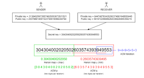Figure 2: Illustration of initial value generation

3.2. Encryption Process

In this design, the image encryption mechanism consists of two main stages, namely, the preparation and manipulation of pixels. In the preparation stage, the image color model is converted to RGBA (red, green, blue, alpha), and the size or dimensions of the image are rectangular. For example, if the original image is 400 × 600, the image will be changed to 600 × 600. The gap between the initial size and the square size (referred to as the border) will be filled with new pixels that have an alpha value of 254, while the original pixel image has an alpha value of 255. Alpha is the channel in the RGBA color model that determines pixel transparency, with a value of 0 indicating transparency and a value of 255 indicating non-transparency. The newly added pixels are given a value of 254 in order to distinguish which pixels are the original pixels in the image and which ones are the border during the decryption process. The newly added pixels have randomly generated values ​​with a range of 0–255. At the pixel manipulation stage, there are two phases: confusion and diffusion. In both phases, several initial value parameters are used. The values ​​for these parameters are obtained through the secret key, as was explained in the previous section.

3.2.1. Confusion Using Arnold’s Cat Map

Confusion is the first pixel manipulation process performed using this image encryption system. Basically, the confusion process involves shuffling or randomizing the position of the pixels comprising the image so that it cannot be recognized anymore. In this design, ACM is used as a chaotic map model to determine the displacement of a pixel.

At the beginning of the formation of ACM, three parameters are needed, namely, p, q, and the number of iterations, which are all positive numbers. The values of the three parameters are obtained from the secret key constituent numbers, as explained in the previous section. The ACM formula is as follows:

where p and q are parameters and N is the size or dimensions of the image. Formula (8) produces a matrix containing  and , which is the new position. For each time this calculation is performed, the pixels in position ,  will be moved to , . This calculation is carried out continuously until all pixels are shuffled. The displacement of pixel positions in the matrix can be performed more efficiently using the meshgrid, which is one of the functions of Python NumPy. First, the meshgrid will be made for x and y with a size of N × N to indicate the original position of the pixels in the image. Then, from the two meshgrids, two xmap and ymap matrices will be formed using formula (8), indicating the new pixel position. Thus, the pixel value at its original position (i.e., [x,y]) will be moved to a new position according to (xmap,ymap). This process will continue to be repeated as many times as the iteration parameter has been set. To ensure that the resulting matrix is ​​more random and difficult to predict, in this design, the values ​​of p and q will vary with each iteration by taking two numbers from the overall values of p and q obtained from the secret key.

3.2.2. Diffusion Using the Henon Map

The main concept of this diffusion process is to perform XOR operations on a matrix of image pixels generated by the confusion process with a chaotic map matrix. This system uses the Henon map as the chaotic map model.

At the beginning of the formation of the Henon map, two initial values are needed, namely  and . Just like in the confusion stage, the two initial values are obtained from the secret key constituent numbers, as explained in the previous section. In this system, the values of  and  are between 0 and 1, with a precision level of . This means that changes in values as small as  can affect the results of the diffusion. In addition to  and , there are other parameters, namely,  and . In this system, the values of  = 1.4 and  = 0.3 are used so that the resulting Henon map is chaotic.

To create a chaotic map, a Henon map formula is calculated with an iteration of  times (  represents the dimensions of the image, and  is the number of bits in each pixel). For example, if the image to be processed is a 512 × 512 8 bpc image, then the iteration will be performed 512 × 512 × 8, or 262,144, times.

For each iteration, new  and  values (  and ) are obtained. From these results, the value of  will be converted to a bit value (0 or 1) using a threshold value of 0.3992 according to the results of [19]. In other words, if the value of  is greater than 0.3992, it will produce a value of 1, but if it is smaller or equal to 0.3992, it will produce a value of 0. Then, the bit will be inserted into the bit sequence. The  and  values generated in the current iteration will be x_n and y_n for the next iteration. At each bpc iteration of a certain multiple, the resulting bit sequence will be converted into a decimal form that will represent the gray value of a pixel. For example, in the 8 bpc image, the bit sequence will be changed to a decimal in the 8th, 16th and 24th iterations, and so on. After all the iterations are finished, a chaotic map will be produced with dimensions .

After the chaotic map is formed, bitwise XOR operations will be performed between the image pixels generated by the confusion process with the chaotic map at the bit level. The results of the XOR operation are stored in a new matrix and become the results of the diffusion process. Diffusion is the last process carried out in this series of encryption processes, so the results are the result of this image encryption system.

3.3. Decryption Process

The flow of decryption is the opposite of encryption, which is divided into undiffusion, unconfusion, and crop border phases. The undiffusion and unconfusion processes involve manipulating image pixels that aim to return the encrypted image pixels to their original values and positions. In both phases, several initial value parameters are used. The values for these parameters are obtained through the secret key, as explained in the previous section. To decrypt the image into its original form, the initial value parameters used in the undiffusion and unconfusion processes must be the same as those used in the diffusion and confusion processes during encryption. Differences in values can cause the image to not be decrypted.

After going through the undiffusion and unconfusion phases, there is one more phase that must be completed, namely, the crop border process. In this phase, the original image has been seen, but the dimensions of the image are still not in accordance with the original due to changes in the image dimensions in the encryption process. Therefore, a crop border is performed to remove the pixels added during the encryption process so that the image returns to its original dimensions.

3.3.1. Undiffusion using the Henon Map

The undiffusion process is the opposite of the diffusion process performed at the time of encryption. If diffusion involves changing the value of the pixels that make up the image, the undiffusion process restores encrypted image pixels to their original values. The approach is the same as that carried out during the diffusion process: one makes chaotic maps and then performs a bitwise XOR operation. This can be done with an XOR operation because of its reversible characteristics. The only difference between the diffusion and undiffusion processes is the operand. During the diffusion process, an XOR operation is performed between the confusion matrix and the chaotic map, whereas in the undiffusion process, an XOR operation is performed between the encrypted matrix and the chaotic map. To restore encrypted image pixels to their original values, the chaotic map used in undiffusion must be the same as that used during the diffusion process. Chaotic map mismatch will cause the pixel values to change from the original values, so the image will not be successfully decrypted.

The unconfusion process is the opposite of the confusion process during encryption. In the confusion process, the original image’s pixel positions are randomized, so the pixel positions in the encrypted image are not the same as in the original image. As for the unconfusion process, the pixel positions in the encrypted image, which have been scrambled, will be returned to their original positions. The formula used for unconfusion is as follows:

By using formula (9), the original position of a pixel is obtained , . Each time this calculation is performed, the value of a pixel at position ,  will be returned to its original position , . The calculation is carried out continuously until all the pixels return to their original positions.

The displacement of pixel positions in the matrix can be performed more efficiently by using a meshgrid, as in the confusion process. First, a meshgrid for x and y of N × N size will be created to indicate the pixel position in the encrypted image. Then, from the two meshgrids, two xmap and ymap matrices will be created using formula (9), indicating the new pixel position. Thus, the pixel at the position of [xmap, ymap] will be moved to the position of [x, y]. This transfer is the reverse of that performed in the confusion process because the purpose of the unconfusion process is to return the pixels in the encrypted image to their original positions. This process will be repeated as many times as the number of iterations that has been set. The number of iterations carried out in the unconfusion process must correspond to the number of iterations performed during the confusion process. Mismatch in p, q, or the number of iterations will cause the pixels in the image to not return to their original positions. Just like in the confusion process, the p and q values ​​in the unconfusion process change with each iteration, but inversely; the p and q values ​​used in the last iteration in the confusion process will be the p and q values ​​of the first iteration in unconfusion, and so on.

3.3.2. Unconfusion using Arnold’s Cat Map

The unconfusion process is the opposite of the confusion process performed during encryption. In the confusion process, the original image’s pixel positions are randomized, so the pixel positions in the encrypted image are not the same as in the original image. As for the unconfusion process, the pixel position in the encrypted image, which have been scrambled, will be returned to their original positions. The formula used in the unconfusion process is as follows:

By using formula (9), the original position of a pixel is obtained , . Each time this calculation is performed, the value of a pixel at position ,  will be returned to its original position , . This calculation is carried out continuously until all the pixels return to their original positions.

The displacement of pixel positions in the matrix can be performed more efficiently by using a meshgrid, as in the confusion process. First, a meshgrid for x and y of N × N size will be created to indicate the pixel position in the encrypted image. Then from the two meshgrids, two xmap and ymap matrices will be created using formula (9), indicating the new pixel position. Thus, the pixel value at the position of [xmap, ymap] will be moved to the position of [x, y]. This transfer is the reverse of that performed in the confusion process because the purpose of the unconfusion process is to return the pixels in the encrypted image to their original positions. This process will be repeated as many times as the number of iterations that has been set. The number of iterations carried out in the unconfusion process must correspond to the number of iterations performed during the confusion process. Mismatch in p, q, or the number of iterations will cause the pixels in the image to not return to their original positions. Just like in the confusion process, the p and q values ​​in the unconfusion process change with each iteration, but inversely; the p and q values ​​used in the last iteration in the confusion process will be the p and q values ​​of the first iteration in unconfusion, and so on.

4.Test and Analysis

4.1. Image Encryption Testing Using Confusion

In this test, encryption was performed on 30 images with only confusion, using ACM as the chaotic map. An example of the encryption result can be seen in Figure 3.

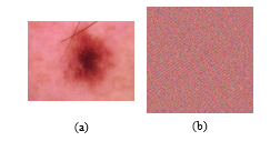Figure 3: (a) Original image and (b) image encrypted using confusion

From the results of this test, we can see that the image does not show the characteristics of the original image because the pixel positions have been shuffled. However, the colors in the encrypted image are the same as the colors in the original image because no pixel values were changed during encryption; new pixels were only added to reshape the image into a square.

In terms of pixel distribution, the histogram generated from 30 encrypted images has the same pixel distribution trend as the original image’s histogram. A comparison between the histograms of the original image and the encrypted image can be seen in Figure 4. Although the trends shown by the two images look similar, it should be noted that the number of pixels is different. In the original image, there are several pixels with a value of 0, whereas in encrypted images there are none. This happens because, during the encryption process, new pixels with random values are added to reshape the image into a square. Thus, the number of pixels considered in the histogram increases. Confusion does not change the pixel values at all, so it does not change the distribution of pixel values in the image. Thus, it can be concluded that the confusion method is not safe enough by itself.

Then, analysis of the correlation between pixels is performed by calculating the correlation coefficients between the neighboring pixels horizontally, vertically, and diagonally. Correlation coefficient values range from -1 to 1, where 1 indicates perfect correlation, 0 indicates no correlation at all, and -1 indicates negative correlation. This calculation is performed three times for each channel (red, green, and blue), and then the average value is calculated. A comparison of the average correlation coefficients of the original image and the encrypted image can be seen in Table 1.

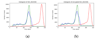Figure 4: Histogram of (a) the original image and (b) the image encrypted using confusion

Based on the average correlation coefficient, the neighboring pixels in the original image have a strong linear correlation, with correlation coefficients close to 0. By contrast, in the encrypted image, the correlation coefficients between neighboring pixels are close to 0. This shows that the confusion method successfully weakens the correlation between neighboring pixels in an image.

Table 1: Comparison of average correlation coefficients of the original image and the image encrypted using confusion

Correlation coeff.	Horizontal	Vertical	Diagonal
Original image	0.984251	0.981887	0.974224
Encrypted image	-0.08009	-0.0462	0.084784

After that, entropy analysis is performed to calculate the level of uncertainty of the pixel values in the encrypted image. The ideal entropy of encrypted image is , which equals 8. A comparison of the average entropy of the original and encrypted images can be seen in Table 2.

We can see that images encrypted with confusion have higher entropy than the original image, with an average entropy value above 7. In theory, confusion should not change the entropy value of the image because there is no change in the pixel value. However, in this test, a greater entropy value was obtained because, during the encryption process, new pixels with random values are added to change the shape of the image into a square. The addition of these random pixels makes the entropy value increase from 6.912776 to 7.401581. Even so, the encrypted image with this entropy value is not secure enough and is still predictable. Encrypted images are considered to be safe if they have an entropy value close to 8, which indicates that the pixels in the image are difficult to predict.

Table 2: Comparison of the average entropy of the original image and the image encrypted using confusion

	Entropy
Original image	6.912776
Encrypted image	7.401581

4.2. Image Encryption Testing Using Diffusion

In this test, encryption was performed on 30 images with only diffusion, using the Henon map as the chaotic map. An example of the encryption results can be seen in Figure 5.

We can see that the image does not represent the original color, but instead consists of a variety of random colors. This is a result of changing the image’s gray values during encryption. Nevertheless, even though it is very vague, the object or shape depicted in the original image is still visible because no randomization of pixel positions was performed during encryption.

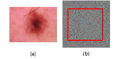Figure 5: (a) Original image and (b) image encrypted using diffusion

In terms of pixel distribution, the histogram of encrypted image is very different from the original image. When viewed as a whole, 30 histograms of encrypted images have the same characteristics; every possible gray value is fairly diffused to all image pixels due to the use of a diffusion method that changes pixel values. An example of a comparison of the original and encrypted images’ histograms can be seen in Figure 6. This is because of the nature of the Henon map, which produces a sequence of random numbers that produces very diverse gray values when an XOR operation is performed on the pixels of the original image.

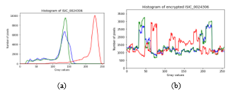Figure 6: Histogram of (a) the original image and (b) the image encrypted using diffusion

Then, the correlation analysis between pixels is performed by calculating the correlation coefficients between the neighboring pixels horizontally, vertically, and diagonally. This calculation is performed 3 times for each channel (red, green, and blue), and then the average value is calculated. A comparison of the average correlation coefficient of the original image and the encrypted image can be seen in Table 3.

From the average correlation coefficient, it can be seen that the neighboring pixels in the image encrypted with diffusion have almost no correlation at all. Indeed, the coefficients are very close to 0, which are even smaller than those for the image encrypted with confusion.

Table 3 Comparison of average correlation coefficient of the original image and the image encrypted using diffusion

Correlation coeff.	Horizontal	Vertical	Diagonal
Original image	0.984251	0.981887	0.974224
Encrypted image	0.000195	-0.00035	-0.00107

After that, entropy analysis is performed to calculate the level of uncertainty of the encrypted image. A comparison of the average entropy of the original and encrypted images can be seen in Table 4. Using the entropy calculation, we can see that encrypted images with diffusion have a much higher entropy than the original image, with an average entropy of 7.950477, which is very close to 8. The entropy value produced in this test is even greater than the entropy value of the image encrypted with confusion in the previous test. This happens because diffusion changes the pixel values, which makes the distribution of pixel values in the image more random. The entropy value of 7.950477 indicates that the pixels in the encrypted image with diffusion are random and difficult to predict.

Table 4 Comparison of the average entropy values of the original image and the image encrypted using diffusion

	Entropy
Original image	6.912776
Encrypted image	7.950477

4.3. Image Encryption Testing Using a Combination of Confusion and Diffusion

In this test, encryption was performed on 30 images with a combination of confusion and diffusion, using ACM and Henon map as the chaotic maps. An example of the encryption results can be seen in Figure 7.

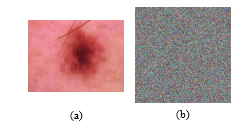Figure 7: (a) Original image and (b) image encrypted using a combination of confusion and diffusion

We can see that image does not represent the original color because the pixel value has been changed at the time of encryption during the diffusion stage. On the other hand, the characteristics of the original image are not visible because the encryption process is done by randomizing the position of the pixel image during the confusion stage.

In terms of pixel distribution, the histogram produced in this test is the same as histogram in test B (diffusion only), although the method used in this test is a combination of confusion and diffusion. An example comparison of the histogram of the original image and the encrypted image can be seen in Figure 7. This can occur because confusion does not change the pixel value, and the value of the pixel changes at only the diffusion stage.

Just like the results of the histogram in test B, all histograms in this test have the same characteristics; every possible gray value is fairly diffused to all pixels in the image due to the use of a diffusion method that changes pixel values. An example comparison of the original and encrypted image histograms can be seen in Figure 8. This is because the Henon map produces a sequence of random numbers, so that very diverse gray values are produced when an XOR operation is performed on the pixels of the original image.

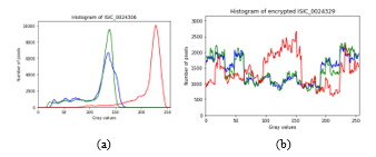Figure 8: Histogram of (a) the original image and (b) the image encrypted using a combination of confusion and diffusion

Then, correlation analysis between pixels is performed by calculating the correlation coefficients between the neighboring pixels horizontally, vertically, and diagonally. This calculation is performed three times for each channel (red, green, and blue), and then the average value is calculated. A comparison of the average correlation coefficient of the original image and the encrypted image can be seen in Table 5.

Based on the average correlation coefficient, which is very close to 0, the neighboring pixels in the image encrypted with only diffusion have almost no correlation at all.

Table 5: Comparison of the average correlation coefficients of the original image and the image encrypted with a combination of confusion and diffusion

Correlation coeff.	Horizontal	Vertical	Diagonal
Original image	0.984251	0.981887	0.974224
Encrypted image	0.003877	-0.00026	-0.00049

After that, entropy analysis is performed to calculate the level of uncertainty of the encrypted image. A comparison of the average entropy values of the original and encrypted images can be seen in Table 6. Based on the entropy calculation, the images encrypted with diffusion have a much higher entropy value (an average of 7.950304, which is very close to 8) than the original image. The entropy value produced in this test is even greater than the value of the image encrypted with only confusion, and it is more or less the same as the value of the image encrypted with only diffusion. This happens because diffusion changes the pixel values, which makes the distribution of pixel values in the image more random. The entropy of 7.950304 indicates that the pixels in the image encrypted with diffusion are random and difficult to be predicted.

Table 6: Comparison of average entropy of original and encrypted images using confusion and diffusion combined

	Entropy
Original image	6.912776
Encrypted image	7.950304

4.4. Image Encryption Testing Using Modified Secret Keys

In this test, IMG_0130 (a photo taken by the clinic) and ISIC_0024306 (a dataset image) are encrypted using the secret key, 646286328968294135017954110561, producing the image shown in Figure 9. This is the original key that will be used for comparison in a key sensitivity analysis. After that, the encryption test was performed again using the 30 modified secret keys. In this system, the secret key is not actually known by the client because it is the result of DH, but to discover the sensitivity of the key used as the initial values for encryption in this test scenario, an encryption test will be performed using a modified secret key.

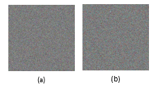Figure 9: Encrypted image: (a) IMG_0130 and (b) ISIC_0024306, which used the original secret key

In each test, the modified secret key is one number different from the original secret key, starting from the largest number ( ) to the smallest ( ), while the other 29 numbers are the same as the original numbers. Variations of the secret key in this test can be seen in Table 7.

Table 7: Modified secret keys

Trial no.	Modification precision	Secret key
1		546286328968294135017954110561
2		636286328968294135017954110561
. .	. .	. .
29		646286328968294135017954110551
30		646286328968294135017954110560

In this test, an analysis is performed by calculating the similarity index (SSIM) to determine the level of similarity between the image encrypted using the original secret key and the one encrypted using the modified secret key. The SSIM index has values ranging from 0 to 1, with 1 meaning that the images are identical or entirely the same. The results of SSIM calculations of the original encryption and encryption with the modified key can be seen in Table 8.

The images encrypted using the original secret key and modified secret key have very significant differences, as indicated by the very small similarity index. In the first 28 trials, which had modification precision of ( ) to ( ), the similarity index results were only around 0.005, or about 0.5%. In contrast, for the secret key modification of the last two numbers, which had levels of precision of ( ) and ( ), the similarity index is around 0.12, or 12%, as the Henon map (diffusion) uses only the first 28 numbers as initial values. Thus, the secret key used to determine the initial values in the encryption process is very sensitive to changes; even the slightest change in the smallest number can generate a completely different image.

Table 8: Similarity index between encrypted image using original secret key and modified secret key

Modification precision	Similarity index (SSIM)		Average
	IMG_0130	ISIC_0024306
	0.00485	0.00556	0.005205
. .	. .	. .	. .
	0.00497	0.00628	0.005625
	0.09249	0.1496	0.121045
	0.09231	0.14984	0.121075
Total Average			0.005337

4.5. Image Decryption Testing Using Modified Keys

Two kinds of tests are conducted. The first is decryption of the encrypted image in Figure 9b using 30 secret keys, as shown in Table 7. These secret keys are modifications of the actual secret key (646286328968294135017954110561). The second test is decryption of the encrypted image in Figure 9b using a public key and a private key. This test was conducted 30 times using 30 private keys, as shown in Table 9. These private keys are modifications of the actual private key (885733484466402526888140697877). The public key used in the tests is always the same (203798914001523740619069244784).

The first test is carried out to determine the secret key’s sensitivity to the resulting encrypted image, while the second test is more like a simulation of image decryption in real circumstances by an attacker (not the actual recipient). This is done because in the image encryption program designed in this research, the user must enter their private key and the sender’s public key to be able to decrypt the image. Therefore, the second test in this test scenario is intended to determine the sensitivity of the private key to the encrypted image that is generated.

Table 9: Modified private keys

Trial no.	Modification precision	Private key
1		785733484466402526888140697877
2		875733484466402526888140697877
. .	. .	. .
29		885733484466402526888140697867
30		885733484466402526888140697876

From the results of the tests that have been carried out, no image has been successfully decrypted to its original form, but in the last two trials of the decryption test with secret key modifications, the decrypted images represent the colors of the original image, which can be seen in Figure 10.

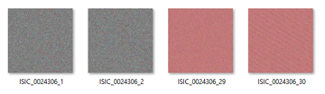Figure 10: The last two trials of the decryption test using the modified secret keys

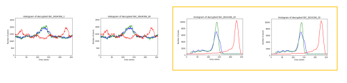Figure 11: Histograms of the decryption results obtained using modified secret keys (1st, 28th, 29th, and 30th trials)

This section analyzes the decryption results with histogram and entropy analysis. Histograms for the decryption test using modified secret keys can be seen in Figure 11. Overall, the histograms show uniform pixel distribution, except for the 29th and 30th trials. This type of pixel distribution is caused by differences between the initial Henon map values ​​used in the encryption and decryption processes. When the initial values used in the decryption process are not the same as those in the encryption process, an entirely different chaotic map is generated rather than restoring the pixels to their original values. In the 29th and 30th experiments, because the initial values of the Henon map used for decryption were the same as the values used for encryption, the trend of pixel distribution matches the original image, indicating that the encrypted pixel values ​​have returned to their original values. Meanwhile, in the ACM, the initial values were not the same, so the pixels in the image did not return to their original positions.

Histograms for the decryption test performed using modified private keys can be seen in Figure 12. From these histograms, we can see that all the trials—both those using the Henon map and ACM—failed to decrypt the image to its original form.

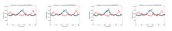Figure 12: Histograms of the decryption results obtained using modified private keys (1st, 28th, 29th, and 30th trials)

Next, entropy analysis was performed to prove that the decryption results are random and difficult to predict. The results of entropy calculations can be seen in Table 10. The failed decryption trial makes the entropy value greater, which means that the image is more random and more difficult to predict. Indeed, the overall entropy is above 7.99, which is very close to 8. However, in the 29th and 30th trials of the secret key modification test, the entropy values of only around 7.54.

Table 10: Entropy of decryption results obtained using modified keys

Trial no.	Image	Entropy
		Modified secret keys	Modified private keys
1	IMG_0130	7.99484	7.9948
. .	. .	. .	. .
28	ISIC_0024327	7.99468	7.9948
29	ISIC_0024328	7.54545	7.99492
30	ISIC_0024329	7.54545	7.99486

Of the two tests that were carried out, the scenario in the second test, in which the encryption system is designed to use both a public key and a private key as well as a secret key that is a combination of both, is more likely to occur in real life. However, it is also possible for the attacker to use direct brute force on the secret key that is generated. Key space analysis is needed to prove that the keys are secure enough.

Both the secret key and the private key in this design consist of decimal numbers with a length of 30 characters. Thus, there are  permutations. Key spaces of this length can overcome brute force attacks.

4.6. Algorithm Complexity Analysis

There are three stages of encryption that are carried out sequentially, namely, reshaping, confusion, and diffusion. During the reshaping phase, the image is converted into a square, adding new pixels to fill in the blanks. Therefore, in this section a random number of N × N is filled in, where N is the largest dimension of the original image. If calculated using Big-O notation, it is O(N²). Then, confusion is performed with several operations:

• Generate a meshgrid of N × N size, calculated as O(N²).
• Loop as many as I iterations, calculated as O(I).
• Take p and q from the secret key, calculated as O(2×1).
• Generate an xmap and ymap by calculating the ACM of the values in the meshgrids x and y, calculated as O(2×N²).
• Move pixels from position (x, y) to position (xmap, ymap), calculated as O(N²).

Throughout this calculation, the constant Big-O notation can be removed from the calculation because of its very small effect compared to O(N²). Therefore, from this confusion stage, we obtain a complexity calculation of O(N²) + O(I) × O(3N²) = O(N²) + O(I × 3N²).

Diffusion is performed as follows:

• Loop as many as N × N × 8 iterations, calculated as O(8N²).
• Calculate xN and yN with the Henon map formula, calculated as O(2×1).
• xN and yN become x and y values for the next iteration, calculated asO(2×1).
• Convert xN to binary bit by using a threshold. In the worst-case scenario, there are four operations that must be performed, so it is calculated as O(4×1).
• Insert binary bits into the bit sequence, calculated as O(1).
• Check whether the current iteration is a multiple of 8, calculated as O(1).
• If it is a multiple of 8, convert the bit sequence into decimal form, empty the bit sequence, and then insert the decimal value into the chaotic matrix. All of these operations are counted as O(3×1).
• After all the iterations are finished, perform an XOR operation between the chaotic matrix and the image matrix for each channel, calculated as O(3×8N²) = O(24N²).

From this confusion phase, we obtain a complexity calculation of O(8N²) × (O(2) + O(2) + O(4) + O(1) + O(1) + O(3)) + O(24N²) = O(132N²). When combined, the entire encryption algorithm has a complexity of O(N²) + O(N²) + O(I × 3N²) + O(132N²), or O(3I+134)N², where I is the number of iterations at the confusion stage and N is the largest dimension of the original image. Based on the complexity notation, the performance and time needed to run the encryption process are influenced by the large number of iterations that must be done at the confusion stage as well as the largest dimension of an image. Of these factors, the largest dimension of the image has the most influence on performance and the time needed to carry out the encryption/decryption process, as indicated by the notation in the form of quadratic time.

The decryption process has more or less the same complexity as the encryption process. The undiffusion and unconfusion stages of decryption perform similar numbers and types of operations to the diffusion and confusion stages of the encryption process, so the complexity calculation is the same. The only difference between decryption and encryption leis in the reshape phase; in the worst-case scenario, the process of returning the image to its original form (crop border) has an operating complexity of O(2N+3N²). Thus, the overall complexity of the decryption algorithm is O(2N+3N²) + O(N²) + O(I × 3N²) + O(132N²), or O(2N + 136N² + I × 3N²).

Overall, there is not much difference between the complexity of encryption and decryption. Similar to the encryption process, the performance and time required to carry out the decryption process are affected by the large number of iterations that need to be performed at the unconfusion stage as well as the length/width of the image to be decrypted. The length/width of the image is the factor with the biggest influence.

5. Conclusions

There are several conclusions that can be made based on the tests conducted in this research:

1. Chaos-based image encryption using only the confusion method is not secure enough, as evidenced by the fact that the pixel distribution trend is similar to the original image and the average entropy value is 7.401581.
2. Chaos-based image encryption using only the diffusion method is secure enough based on the distribution of pixels on the histogram, the average correlation coefficient (which is very close to 0), and the average entropy (7.950477). However, the characteristics of the original image are still vaguely visible.
3. Chaos-based image encryption using a combination of confusion and diffusion methods is the most secure encryption method based on pixel distribution on the histogram, the average correlation coefficient (which is very close to 0), and the average entropy (7.950304). Implementing two methods is more secure because there are two layers of security.
4. Implementation of ACM in the confusion phase with different p and q values ​​in each iteration makes pixel positions more random and difficult to predict.
5. The initial values of the Henon map have a sensitivity level of at least .
6. A difference of just one number in the secret key during the encryption process results in a significant difference in the encrypted image, as evidenced by the average similarity level of around 0.5%. This indicates that changes in the initial values ​​of the ACM or Henon map can make a big difference in the encryption results.
7. A difference of just one number in the secret key during the decryption process causes the image to not be restored to its original shape and produces a stronger random image with entropy values closer to 8.
8. A 30-character numeric key has a high level of security because there are permutations that might be generated.
9. The largest dimension of an image (length/width) is the factor with the most influence on the performance and time involved in running the encryption/decryption process.

Acknowledgment

This research is supported and funded by Directorate of Research and Community Service, Deputy for Strengthening Research and Development, Ministry of Research, Technology / National Research and Innovation Agency of the Republic of Indonesia under the grant of Penelitian Konsorsium Riset Unggulan Perguruan Tinggi 2020, contract number: Nomor: 2115/PKS/ITS/2020.

1. S.S. Alwy, KONSIL KEDOKTERAN INDONESIA, 2006.
2. D. Desai, A. Prasad, J. Crasto, “Chaos-Based System for Image Encryption,” 3(4), 4809–4811, 2012.
3. S. Fadhel Hamood, M.S. Mohd Rahim, O. Farook Mohammado, “Chaos image encryption methods: A survey study,” Bulletin of Electrical Engineering and Informatics, 6(1), 99–104, 2017, doi:10.11591/eei.v6i1.599.
4. A. Soleymani, M.J. Nordin, E. Sundararajan, “A chaotic cryptosystem for images based on Henon and Arnold cat map,” Scientific World Journal, 2014, 2014, doi:10.1155/2014/536930.
5. Diffie-Hellman Protocol — from Wolfram MathWorld, Dec. 2019.
6. L. Kocarev, “Chaos-based cryptography: A brief overview,” IEEE Circuits and Systems Magazine, 1(3), 6–21, 2001, doi:10.1109/7384.963463.
7. Y. Kumar, S. Mamta, “A Review Paper on Image Encryption Techniques,” International Journal for Research in Applied Science & Engineering Technology, 5(4), 169–172, 2014, doi:10.22214/ijraset.2017.8023.
8. N.A. Abbas, “Image encryption based on Independent Component Analysis and Arnold’s Cat Map,” Egyptian Informatics Journal, 17(1), 139–146, 2016, doi:10.1016/j.eij.2015.10.001.
9. E. Hariyanto, R. Rahim, “Arnold’s Cat Map Algorithm in Digital Image Encryption,” International Journal of Science and Research (IJSR), 5(10), 1363–1365, 2016, doi:10.21275/ART20162488.
10. F.J. Dyson, H. Falk, “Period of a Discrete Cat Mapping,” The American Mathematical Monthly, 99(7), 603, 1992, doi:10.2307/2324989.
11. M.F. Abd Elzaher, M. Shalaby, S.H. El Ramly, “An arnold cat map-based chaotic approach for securing voice communication,” in The 10th International Conference on Informatics and Systems, Giza: 329–331, 2016, doi:10.1145/2908446.2908508.
12. A.M. Elshamy, M.A. Abdelghany, A.Q. Alhamad, H.F.A. Hamed, H.M. Kelash, A.I. Hussein, “Secure VoIP System Based on Biometric Voice Authentication and Nested Digital Cryptosystem using Chaotic Baker’s map and Arnold’s Cat Map Encryption,” in 2017 International Conference on Computer and Applications, ICCA 2017, Doha: 140–146, 2017, doi:10.1109/COMAPP.2017.8079739.
13. C. Saha, M.F. Hossain, “MRI Watermarking Technique Using Chaotic Maps, NSCT and DCT,” in 2nd International Conference on Electrical, Computer and Communication Engineering, ECCE 2019, IEEE, Cox’s Bazar, 2019, doi:10.1109/ECACE.2019.8679464.
14. N. Lazarov, Z. Ilcheva, “A fragile watermarking algorithm for image tamper detection based on chaotic maps,” in 2016 IEEE 8th International Conference on Intelligent Systems, IS 2016 – Proceedings, Sofia: 723–728, 2016, doi:10.1109/IS.2016.7737391.
15. R. Munir, “A Secure Fragile Video Watermarking Algorithm for Content Authentication Based on Arnold Cat Map,” in 2019 4th International Conference on Information Technology (InCIT), IEEE, Bangkok: 32–37, 2019.
16. Hénon Map — from Wolfram MathWorld, Dec. 2019.
17. N.S. Raghava, A. Kumar, “Image Encryption Using Henon Chaotic Map With Byte Sequence,” 3(5), 11–18, 2013.
18. J. Lin, X. Si, “Image encryption algorithm based on hyperchaotic system,” in 2009 International Workshop on Chaos-Fractals Theories and Applications, IWCFTA 2009, 153–156, 2009, doi:10.1109/IWCFTA.2009.39.
19. D. Erdmann, S. Murphy, “Henon Stream Cipher,” Electronics Letters, 28, 9.
20. D. Gollman, Computer Security Third Edition, 2011, doi:10.1017/CBO9781107415324.004.
21. J.G. Sekar, C. Arun, “Comparative performance analysis of chaos based image encryption techniques,” Journal of Critical Reviews, 7(9), 1138–1143, 2020, doi:10.31838/jcr.07.09.209.
22. A. Afifi, “A Chaotic Confusion-Diffusion Image Encryption Based on Henon Map,” International Journal of Network Security & Its Applications, 11(4), 19–30, 2019, doi:10.5121/ijnsa.2019.11402.

(Click Here)

(Click Here)