1.Introduction

Air quality is a measure of how much air is free from pollution and not harmful when inhaled by humans [1]. Air is stated to be polluted when it contains substances or energy, and other components that exceeds the quality standard [2]. Meanwhile, the sources of air pollution can come from natural processes or human activities (anthropogenic), and the air that is soiled by pollutants causes its quality to be poor. In fact, air pollution can have a serious impact on environmental damage, human health, and ecological balance [3]. This can be formed from chemical reactions with other pollutants and physical elements in the atmosphere.

According to The Environmental Protection Agency (EPA), 6 types of air pollutants can cause serious impacts on health and environmental damage, namely CO, NO₂, Pb, PM, O₃, and SO₂ [4]. Therefore, monitoring air pollution is very necessary, because the data obtained can provide a lot of information about air quality in an area and within a certain time. REAS (Regional Emissions inventory in Asia) is an emission inventory owned by the Frontier Research Center for Global Change (FRCGC), Japan Agency for Marine-Earth Science and Technology (JAMSTEC), which provide data sets and various information about air emissions in the Asian region [5]. Furthermore, the REASv3.1 (latest version) provides complete anthropogenic emission data for the period of 1950 – 2015.

The three anthropogenic emissions that causes respiratory problems, such as airway irritation, bronchitis, asthma, and pneumonia, are NO_X, SO₂, and PM [6–8]. The spread of these emissions is very broad, fast, and has a direct impact on health and the environment [9]. In Indonesia, complete and up to date NO_X and SO₂ emission data is rather difficult to obtain, because many ISPU stations (Air Pollutant Standard Index) that are tasked with monitoring air pollution are not operating properly. Therefore complete data on air emissions in Indonesia are mostly obtained on websites of global emission data providers, even until 2015. This data can be used to analyze air quality trends, and as a basis for forecasting data for 2016 – 2020. Trend analysis is an empirical approach used to determine changes in the values of random variables, whether increasing or decreasing over a period of time in statistical terms. In addition to knowing future air quality conditions, forecasting air emission data is often used to anticipate risks in the event of exposure to poor air quality, as well as to formulate environmental pollution control strategies. [10,11].

Therefore, this research aimed to (1) analyze trends and forecasts of total NO_X and SO₂ emissions in Indonesia from 1950 – 2015, and to compare the methods used to determine the best-performing methods, (2) perform smoothing and forecasting of the dominant sector data from NO_X and SO₂, as well as compare the means used to find out which method has the best performance.

2. Materials and Methods

This study used data from REAS (Regional Emission inventory in Asia) ver.3.1. The data include 10 types of air pollutants (BC, CO, CO₂, NH₃, NO_X, NMNVOC, OC, PM_2.5, PM₁₀, and SO₂), as well as emission sources, both from the producing sector and the type of fuel used [12]. The data used are 2 types of pollutants (NO_X and SO₂), and the 2 largest emission-producing sectors of each pollutants types.

In this research, air emission data processing used two methods, namely the smoothing method with Double Moving Average (DMA) and Double Exponential Smoothing (DES) for emission data per sector. Furthermore, trend analysis was conducted with the exponential approach and polynomial orders of 2 and 3 for total emissions data. Meanwhile, to determine the accuracy of both methods, the results were validated using the calculation of MAD (Mean Absolute Deviation), RMSE (Root Mean Squared Error), and MAPE (Mean Absolute Percentage Error) [13].

where      is the real data of each emission

                 is forecasting data

                  n is the amount of data used.

The focus of this study is in Indonesia, and the research methodology can be seen in Figure 1.

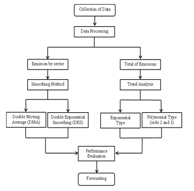Figure 1: Flow diagram of research on forecasting air emission data

To determine the MAPE accuracy criteria, it can be referred to Table 1

Table 1: The accuracy criteria of MAPE [14]

Criteria	The limit of MAPE percentage
Very Good	<10%
Good	10% – 20%
Enough	20% – 50%
Not Accurate	>50%

All data were processed using the Analysis Toolpak, which is a set of “data analysis” tools in the processing group in Microsoft Excel.

The last stage was forecasting data for the next 5 years, starting from 2016 – 2020. For DMA and DES, data forecasting was performed only for the best performance based on the values of MAD, RMSE, and MAPE that met the criteria. For trend analysis, data forecasting was carried out based on the line equation formed from the approach used.

3.     Result and Discussion

3.1. Trend analysis of air pollutants (NO_X, and SO₂)

Estimation or forecasting of total emission data from NO_X and SO₂ pollutants in the coming year was carried out using trend analysis with three approaches, namely, exponential, polynomial order 2, and order 3. Furthermore, the selection of this approach was based on the suitability of the graphical patterns formed between real data and the 3 approaches.

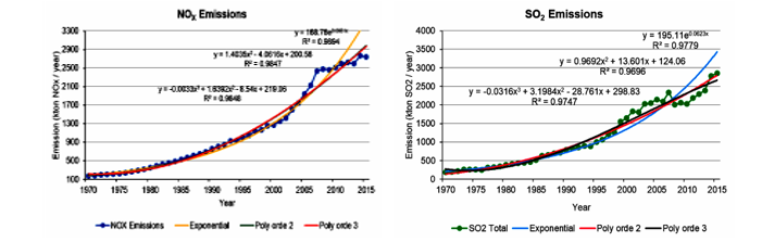Figure 2: Graph of trend analysis for NO_X and SO₂ emissions

Table 2: The validity calculation on the trends analysis results of the NO_X and SO₂ emission

Perform. evaluation	NOX Emission			SO2 Emission
	Exponential	Polynomal		Exponential	Polynomal
		Orde 2	Orde 3		Orde 2	Orde 3
MAD	99.43	69.37	71.99	158.38	108.78	102.78
RMSE	186.91	107.19	107.03	246.07	143.19	130.65
MAPE	7.74	5.77	6.65	10.23	10.19	10.21

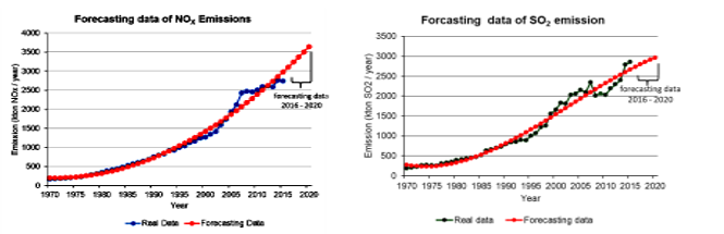Figure 3: Graph of forecasting data for NO_X and SO₂ emissions in period 1970 – 2020

Table 3: The result of forecasting data for NO_X and SO₂ emissions in the period of 2016 – 2020

Year	Total of NOX emission (kton/year)	Total of SO2 Emission (kton/year)	Ratio SO2/NOX
	Polynomial orde 2	Polynomial orde 3
2016	3110.0	2731.5	0.878
2017	3239.3	2792.7	0,862
2018	3371.4	2851.2	0.846
2019	3506.3	2906.8	0.829
2020	3643.9	2959.3	0.812

This study used a lot of data obtained in the period of 1970-2015 or about 45 years. This relatively large data can provide accurate results to minimize errors. Furthermore, this study validated the results using MAD, RMSE, and MAPE to determine the best measurement accuracy of the approach used. Figure 2 showed a graph of trend analysis results on both pollutants, whereas Table 2. showed the performance evaluation results of both graphs

Based on the data validity evaluation, the trend analysis that showed the best performance is the smallest MAD, RMSE, and MAPE values. For NO_X emissions, the use of polynomial order 2 produced a good performance, while for SO₂ emissions, it used a polynomial order 3. Based on the MAPE value, the accuracy of NO_X emission measurements was in the very good category because the value was <10% (5.77%). Meanwhile, for SO₂ emission, it was in a good category because the MAPE value was >10% (10.21%).

For the next stage, the research forecasted data for the next 5 years, between 2016 – 2020, based on graphical equations that have been obtained from trend analysis that showed its best performance. NO_X emission used a polynomial order 2 graph, while SO₂ emission used order 3. The graph equation used for data forecasting was

Forecasting data were obtained by entering x = 1 to represent 1970, x = 2 for 1971, until x = 50 for 2019, and x = 51 for 2020 in equations (4), and (5).

Figure 3 showed the results of forecasting NO_X and SO₂ emission data for the period of 1970 – 2020. Figure 3 showed that in Indonesia, there is an upward trend in emissions for both types of pollutants. This is different from what happened in developed countries, where NO_X and SO₂ emissions showed a downward trend, even though there was growth in the economic and industrial sectors [15]. The quantization graph of forecasting emissions of both pollutants in numerical data can be seen in Table 3, which showed the forecasting results of both pollutants for the period of 2016-2020. Meanwhile, SO₂ emission is only 227.8 tons/year. This means that the NO_X emission gain is more than two times the gain of SO₂. Furthermore, the SO₂ / NO_X ratio has decreased from 0.878 in 2016 to 0.812 in 2020. This showed that the contribution of SO₂ emissions to air pollution in Indonesia is not too significant compared to NO_X

3.2. Smoothing and forecasting data of NO_X and SO₂ emissions

NO_X and SO₂ emission data in this article were collected from 1970 – 2015, and were obtained from REAS version 3.1 [16]. Furthermore, the research smoothed the data for the two dominant sectors in each type of emission. The dominant sectors for NO_X emissions are Road Transportation (Road) and Power Plant (PP), while for SO₂ emissions are Power Plant (PP) and Industry (IND).

Data smoothing is a method used to reduce randomness from time-series data in order to obtain relatively regular data [17,18]. The data smoothing in this research used the Double Moving Average (DMA) and Double Exponential Smoothing (DES) technique. In the DMA technique, 3 variations of the interval were used, namely n = 1, n = 2 and n = 3, while DES used 3 weight variations, namely a = 0.2, a = 0.4, and a = 0.5.

3.2.1. NO_X emissions

Figure 4 showed the results of the smoothing of NO_X emissions data using DMA and DES techniques, for each sector.

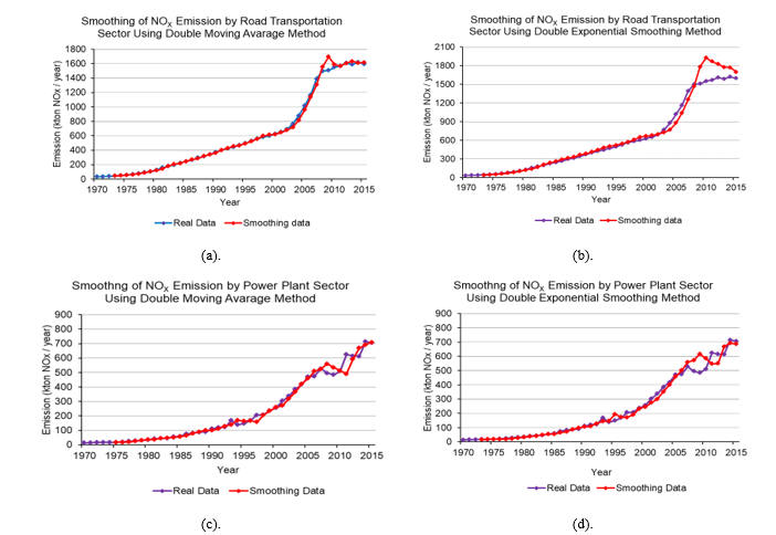Figure 4: Graph of NO_x emission data smoothing for (a). Road sector using DMA (b). Road sector using DES,

(c). PP sector using DMA and (d). PP sector using DES

Table 4: validation of data smoothing for NO_X emissions using the DMA and DES methods.

Double Moving Average (DMA) Method					Double Exponential Smoothing (DES) Method
Road Transportation (Road) sector					Road Transportation (Road) sector
	n=2	n=3	n=4			a=0.2	a=0.4	a=0.5
MAD	17,81	26,11	37,21		MAD	70,64	59,74	58,74
RMSE	36,46	50,98	68,06		RMSE	118,85	102,77	104,58
MAPE	2,72	3,58	4,66		MAPE	14,09	8,26	7,65
Power Plant (PP) sector					Power Plant (PP) sector
	n=2	n=3	n=4			a=0.2	a=0.4	a=0.5
MAD	19,99	15,10	16,81		MAD	26,47	20,87	22,44
RMSE	34,18	28,41	27,42		RMSE	36,06	34,19	39,97
MAPE	8,38	6,68	6,93		MAPE	14,34	9,39	9,53

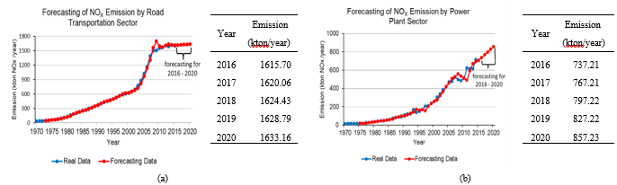Figure 5: Forecasting data of NO_X emissions (a). by road transportation sector and (b). by power plant sectors

To determine the data smoothing performance, the study validated the results obtained. Table 4 showed the performance validation results based on the MAD, RMSE, and MAPE measurements.

Figure 5 showed forecasting NO_X emission data for the Road and PP sectors in the 2016-2020 period. This data forecasting was based on the best performance obtained, namely at n = 2 (Road) and n = 3 (IND).

Table 4 showed that data smoothing using the DMA was better than the DES methods. This can be seen from the smaller MAD, RMSE, and MAPE values for the DMA than the DES methods. For the road transportation sector, the best performance was in the 2 (n = 2) interval, while for the power plant, it was in the 3 (n = 3) interval. For the MAPE value, NO_X emission measurement in the road transportation sector was 2.72%, while the power plant sector was 6.68%. Therefore, the accuracy was in the very good category because the value was <10%.

Figure 5 showed that the forecasting graph for the transportation sector in 2016-2020 is relatively constant or the changes are not too significant, with a gain of 17.46 kton / year. Meanwhile, the power plant sector showed a significant increase with a gain of 120.02 kton / year

3.2.2. SO₂ emissions

Figure 6 showed the results of smoothing SO₂ emission data using DMA and DES techniques for the power plant (PP) and the industrial sectors (IND). The results of smoothing the data from the two methods were then validated using MAD, RMSE, and MAPE. Subsequently, the results were compared to determine the best performance. Table 5 showed the validation results of both methods used

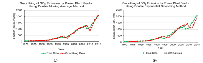
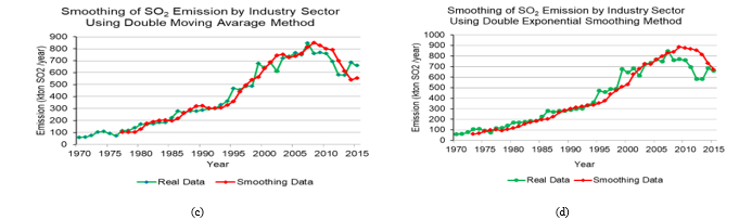Figure 6: Graph of SO₂ emission data smoothing for (a). PP sector using DMA (b). PP sector using DES,

(c). IND sector using DMA and (d). IND sector using DES

Table 5: Validation of data smoothing for SO₂ emissions using the DMA and DES methods.

Double Moving Average (DMA) Method					Double Exponential Smoothing (DES) Method
Power Plant (PP) sector					Power Plant (PP) sector
	n=2	n=3	n=4			a=0.2	a=0.4	a=0.5
MAD	44,85	49,67	60,42		MAD	98,25	83,24	78,91
RMSE	74,06	90,77	106,36		RMSE	148,86	133,14	131,30
MAPE	8,41	8,89	9,75		MAPE	16,79	13,52	13,56
Industry (IND) sector					Industry (IND) sector
	n=2	n=3	n=4			a=0.2	a=0.4	a=0.5
MAD	44,06	41,56	36,00		MAD	50,89	54,40	61,13
RMSE	60,01	60,78	53,33		RMSE	79,32	73,14	82,71
MAPE	11,54	11,25	8,45		MAPE	13,54	14,87	16,81

Table 5 showed that the best performing data smoothing for the PP and IND sectors using DMA was at n = 2 and n = 4, while for DES, it lies at weights a=0.4 and a=0.2. When the results are compared, the DMA method was better than DES, because the values of MAD, RMSE, and MAPE were smaller. For MAPE, the measurement of SO₂ emissions in the power plant sector had a value of 8.41%, while the industrial sector was 8.45%. Therefore, the accuracy was in the very good category because the value was <10%.

Forecasting data for SO₂ emissions in the Road and PP sectors in the 2016 – 2020 period can be seen in Figure 7. This forecasting is based on the best performance obtained, namely at n = 2 (PP) and n = 4 (IND). Figure 7 showed that the data forecasting graph for the power plant sector in 2016-2020 has increased significantly with a gain of 798.5 kton / year, while for the industrial sector showed a decline with a gain of -73.54 kton/year.

In 2015, the installed power capacity for Steam Power Plants (PLTU) was around 53.1% of the total power generation in Indonesia [19]. This showed that the need for coal fuel to supply PLTU needs is very large. Furthermore, the increase in the amount of coal is proportional to the increasing demand for electricity. Therefore, SO₂ gas pollution in the period of 2016 – 2020, appears to have increased significantly. In contrast to the power plant, SO₂ emissions in the industrial sector have decreased, because many industries have implemented the clean production principle by reducing the use of coal as their industrial fuel [20].

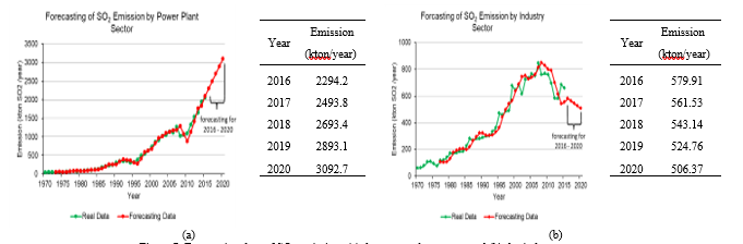Figure 7: Forecasting data of SO₂ emissions (a). by power plant sector and (b). by industry sector

4. Conclusions

4.1.1. The use of Double Moving Average (DMA) method in smoothing NO_X and SO₂ emission data is better than the Double Exponential Smoothing (DES). This is based on the validation results of both methods, where the MAD, RMSE, and MAPE values for the DMA method are smaller than DES. For NOx and SO₂ emissions, the resulting MAPE value in the DMA method was in the very good category, because the value was <10%. Furthermore, the best variation of the moving average interval for NO_X emissions lies at n = 2 (road transportation sector) and n = 3 (power plant sector), while for SO₂ emissions, it lies at n = 2 (power plant sector) and n = 4 (Industry sector).

The forecasting stage for the period of 2016 – 2020 generally showed that the total emissions of NO_X and SO₂ have increased, with the gains for each emission being 533.9 kton / year and 227.8 kton / year. This means that the total emission gain of NO_X is two times greater than SO₂. Furthermore, in the road transportation sector that produces NO_X emissions, changes are not too big, with an emission gain of 17.46 kton / year. Meanwhile, in the power plant sector, it has a quite significant increase, with an emission gain of 120.02 kton / year. SO₂ emissions showed that there is an increase in emissions of power plant sector with a gain of 798.5 kton / year, while for the industrial sector, there is a decrease with a gain of -73.54 kton / year. In addition, the reduction in SO₂ emissions in the industrial sector showed that there is an industrial policy to reduce the use of coal as its energy source.

Conflict of Interest

The authors declare no conflict of interest.

Acknowledgment

The authors would like to thank the Education Fund Management Institute, Ministry of Finance of the Republic of Indonesia, who funded this research.

1. R. Lanzafame, P. Monforte, G. Patanè, S. Strano, “Trend analysis of Air Quality Index in Catania from 2010 to 2014,” Energy Procedia, 82, 708–715, 2015, doi:10.1016/j.egypro.2015.11.796.
2. State Minister of Environment, Regulation of State Minister of the environment Number 12 of 2010 About Regional Air Pollution Control Implementation, 1–199, 2010.
3. G.S. Ajmani, H.H. Suh, J.M. Pinto, “Effects of Ambient Air Pollution Exposure on Olfaction: A Review,” Environmental Health Perspectives, 124(11), 1683–1693, 2016, doi:10.1289/EHP136.
4. R. Williams, V. Kilaru, E. Snyder, A. Kaufman, T. Dye, A. Rutter, H. Hafner, Air Sensor Guidebook, EPA (Environmental Protection gency) USA, 2014.
5. Frontier Research Center for Global Change (FRCGC), Atmospheric Composition Research Program, Http://Www.Jamstec.Go.Jp/Frsgc/Research/P3/Emission.Htm, 2004.
6. H. Yin, M. Pizzol, L. Xu, “External costs of PM2.5 pollution in Beijing, China: Uncertainty analysis of multiple health impacts and costs,” Environmental Pollution, 2017, doi:10.1016/j.envpol.2017.02.029.
7. A.J. Cohen, M. Brauer, R. Burnett, H.R. Anderson, J. Frostad, K. Estep, K. Balakrishnan, B. Brunekreef, L. Dandona, R. Dandona, V. Feigin, G. Freedman, B. Hubbell, A. Jobling, H. Kan, L. Knibbs, Y. Liu, R. Martin, L. Morawska, C.A. Pope, H. Shin, K. Straif, G. Shaddick, M. Thomas, R. van Dingenen, A. van Donkelaar, T. Vos, C.J.L. Murray, M.H. Forouzanfar, “Estimates and 25-year trends of the global burden of disease attributable to ambient air pollution: an analysis of data from the Global Burden of Diseases Study 2015,” The Lancet, 389(10082), 1907–1918, 2017, doi:10.1016/S0140-6736(17)30505-6.
8. N. Sharma, S. Taneja, V. Sagar, A. Bhatt, “Forecasting air pollution load in Delhi using data analysis tools,” Procedia Computer Science, 132, 1077–1085, 2018, doi:10.1016/j.procs.2018.05.023.
9. J. Liu, Y. Chen, T. Lin, C. Chen, P. Chen, T. Wen, C. Sun, J. Juang, J. Jiang, “An air quality monitoring system for urban areas based on the technology of wireless sensor networks,” International Journal On Smart Sensing and Intelegent System, 5(1), 191–214, 2012.
10. W.F. Ryan, “The air quality forecast rote: Recent changes and future challenges,” Journal of the Air and Waste Management Association, 66(6), 576–596, 2016, doi:10.1080/10962247.2016.1151469.
11. A. Jaiswal, C. Samuel, V.M. Kadabgaon, “Statistical trend analysis and forecast modeling of air pollutants,” Global Journal of Environmental Science and Management, 4(4), 427–438, 2018, doi:10.22034/gjesm.2018.04.004.
12. J. Kurokawa, T. Ohara, “Long-term historical trends in air pollutant emissions in Asia: Regional Emission inventory in ASia (REAS) version 3.1,” Atmospheric Chemistry and Physics, 1–51, 2019, doi:10.5194/acp-2019-1122.
13. N.H.A. Rahman, M.H. Lee, Suhartono, M.T. Latif, “Evaluation performance of time series approach for forecasting air pollution index in Johor, Malaysia,” Sains Malaysiana, 45(11), 1625–1633, 2016.
14. D. Febrian, S.I. Al Idrus, D.A.J. Nainggolan, “The Comparison of Double Moving Average and Double Exponential Smoothing Methods in Forecasting the Number of Foreign Tourists Coming to North Sumatera,” Journal of Physics: Conference Series, 1462(1), 2020, doi:10.1088/1742-6596/1462/1/012046.
15. C.S. Lee, K.H. Chang, H. Kim, “Long-term (2005–2015) trend analysis of PM2.5 precursor gas NO2 and SO2 concentrations in Taiwan,” Environmental Science and Pollution Research, 25(22), 22136–22152, 2018, doi:10.1007/s11356-018-2273-y.
16. J. Kowara, T. Ohara, Gridded Data Sets (Information for Data), Https://Www.Nies.Go.Jp/REAS/Index.Html#data%20sets, 2019.
17. S. Bi, S. Bi, D. Chen, J. Pan, J. Wang, “A double-smoothing algorithm for integrating satellite precipitation products in areas with sparsely distributed in situ networks,” ISPRS International Journal of Geo-Information, 6(1), 2017, doi:10.3390/ijgi6010028.
18. T.C. Pataky, M.A. Robinson, J. Vanrenterghem, J.H. Challis, “Smoothing can systematically bias small samples of one-dimensional biomechanical continua,” Journal of Biomechanics, 82, 330–336, 2019, doi:10.1016/j.jbiomech.2018.11.002.
19. Badan Pusat Statistik (BPS), Generating capacity installed by power plant in Indonesia, Http://Www.Bps.Go.Id, 2020.
20. J.M. Grether, N.A. Mathys, J. de Melo, “Global manufacturing SO2 emissions: Does trade matter?,” Review of World Economics, 145(4), 713–729, 2010, doi:10.1007/s10290-009-0033-2.

(Click Here)

(Click Here)

No. of Downloads Per Month

No. of Downloads Per Country